Contributions to Variation in Fly Ball Distances
Back in early 2013, I wrote a guest article for Baseball Prospectus entitled “How Far Did That Fly Ball Travel?” In that article, I posed a seemingly simple question: Can we predict the landing point of a fly ball just after it leaves the bat? A more precise way to ask the question is as follows: Suppose the velocity vector of a fly ball just after leaving the bat is known, so that the exit velocity, launch angle, and spray angle are all known. How well does that information determine the landing point? I then proceeded to investigate the question, at least for home runs, with the aid of HITf/x data for the initial velocity vector and the ESPN Home Run Tracker for the landing point and hang time. Using a technique described in the article, that information was used along with a trajectory model to reconstruct the full trajectory and extrapolate it to ground level to determine the fly ball distance. The answer to the question was immediately obvious: The initial velocity vector poorly determines the fly ball distance.
This conclusion led naturally to the next question: Why? One obvious reason is variation in atmospheric conditions, especially wind. However, the data revealed that the variation in home run distance for given initial velocity was as large in Tropicana Field, where the atmospheric conditions are expected to be constant, as in the rest of the league. So that was eliminated, at least as the primary culprit.
The article then went on to consider variation in two other parameters that play a role in fly ball distance: backspin ωb and drag coefficient CD. Neither of these parameters were directly measured. Rather they were inferred, along with the sidespin ωs, in the procedure used to recreate the full trajectory. The analysis showed the following:
- For a given value of CD, distance increases as ωb increases. This makes sense, since larger backspin results in greater lift, keeping the ball in the air longer so that it travels farther.
- For a given value of ωb, distance decreases as CD increases. Again this makes sense, since greater drag is expected to reduce the carry of a fly ball. Interestingly, this was the first appearance in print of a suggestion of a significant ball-to-ball variation in the drag properties of baseballs.
- There was a moderately strong positive correlation between CD and ωb, suggesting that the drag on a baseball increases with increasing spin, all other things equal. Although this effect is well known for golf balls and had been speculated for baseballs in R. K. Adair’s excellent The Physics of Baseball, to my knowledge this is the first real evidence showing the effect for baseballs.
- Given that both lift and drag increase with increasing ωb and that they have the opposite effect on distance, it was tentatively concluded that at high enough spin rate there would be no further increase (and perhaps even a decrease) in distance with a further increase in spin.
Given the above conclusions, which were based on indirect determinations of spin and drag, I decided that it was necessary to do a dedicated experiment under controlled conditions. That led to the January 2014 Minute Maid Park experiment done by my Washington State collaborators, my student, and me under controlled atmospheric conditions, leading to another article. In the experiment, we had complete control over the initial exit velocity, launch angle, and backspin using a specially designed ball launcher. Further, we utilized the stadium Trackman to obtain the full trajectory for each fly ball, from which we could unambiguously determine the drag coefficient. The experiment confirmed directly all of the conclusions reached indirectly from the previous home run analysis, particularly:
- A significant ball-to-ball variation in CD for fixed ωb.
- An increase in CD with ωb.
- Remarkably little variation in fly ball distance for backspins in the range 2000-3200 rpm.
Interestingly, neither of these studies considered the effect of either the spray angle or sidespin ωs on the carry of a fly ball. Both those issues were addressed in my more recent unpublished article, “Why Does a Fly Ball Carry Better to Centerfield?”. From analysis of Statcast data, including exit velocity, launch angle, spray angle, backspin rate, sidespin rate, and distance, the following was found:
- Fly ball distance depends on ωs, which in turn depends on the spray angle. Therefore, fly ball distance depends on the spray angle.
- Fly ball distance is largest when ωs=0 and is roughly symmetric about ωs=0.
- ωs=0 (and therefore fly ball distance is maximum) at a spray angle slightly to the pull side of straightaway center field.
- As a consequence of the previous bullet point, balls hit at a given spray angle to the pull side (where the magnitude of ωs is smaller) will carry farther than balls hit at the same spray angle on the opposite side (where the magnitude of ωs is greater).
These observations make it clear that my earlier work needs to be expanded to include the effects of spray angle and sidespin, leading to the present analysis. The earlier observation was that for fixed exit velocity and launch angle, there was a variation in fly ball distance. The list of possible factors will now include the following: φ∗, ωb, ωs, CD, and measurement noise. The goal will be to quantitatively determine the contribution of each of these to the variation in fly ball distance.
Statcast Data
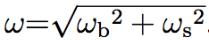
The data used in this study are Statcast batted ball trajectories from the 2016-2019 seasons. As in the earlier study, the data include exit velocity v0, launch angle θ, adjusted spray angle φ∗, and landing location. However, unlike the earlier study, the data consist of actual trajectories rather than a model for the trajectories, thereby improving considerably the ability to determine the drag coefficient CD. The data also include the spin rate ω and spin axis, from which a separation of ω into backspin ωb and sidespin ωs rates can be done. (Here it should be noted that while the Trackman radar system, an integral part of Statcast, measures the total spin ω directly, it only infers the spin axis (and therefore ωb and ωs) from the trajectory, using a proprietary algorithm.) Once again, this is an improvement over the previous study in which the spin components were inferred but not measured.
Only fly balls were chosen for which the batted ball was tracked to at least 80% of its eventual distance, assuring good precision in determining the full distance by extrapolating the trajectory to ground level. Moreover, only data from Tropicana Field were utilized, thereby assuring stable atmospheric conditions. The data were restricted to exit velocities in the range 94-110 mph and launch angles in the range 25-30 degrees, resulting in a total of 719 fly balls, with distances in the range 320-460 feet.
Analysis
The analysis reported here is a bit tricky because some of parameters being investigated are coupled to each other. For example, ωs (and to a lesser extent ωb) both depend on φ∗. Moreover, CD depends on the total spin
Given these dependencies, the analysis proceeds as follows.
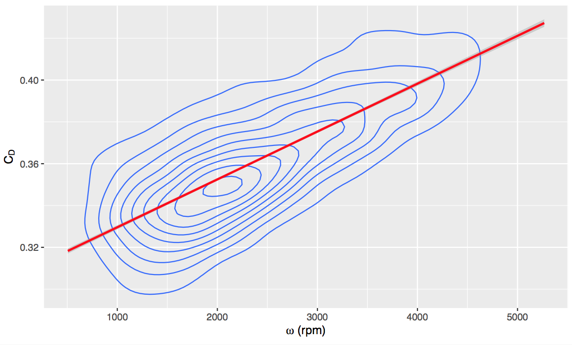
The first step will be to determine CD from the rising segment of trajectory using techniques that are described in Appendix C of the report of the MLB Home Run Committee. The next step is to determine the linear dependence of CD on ω, which is shown in Figure 1 and has a slope α=(2.45 ± 0.09) × 10−5 rpm−1. Then for each batted ball event, the spin- independent drag coefficient CD0 is found, where
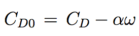
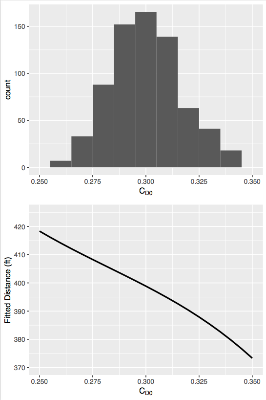
This quantity is approximately normally distributed with standard deviation 0.018 (see Fig. 3), which is interpreted to be the ball-to-ball variation in drag coefficient, with the effect of spin removed. It is one of the factors contributing to the variation in fly ball distance.
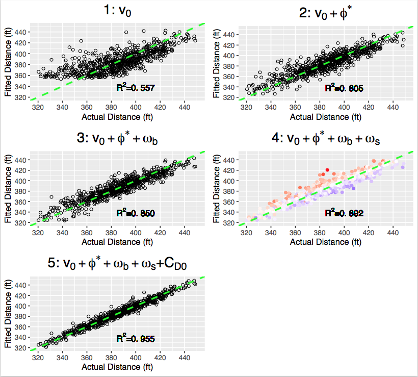
The next step is to perform a sequence of fits to the distance data using a non-parameteric generalized additive model, with each step in the sequence controlling for an additional parameter. In that manner, the effect of the added parameter on the fit can be determined, for fixed values of all the preceding parameters. In each fit, the launch angle is essentially a fixed parameter given its narrow range at the flat part of the distance-vs-θ distribution. The results of this procedure are given in Table I.
Model 1 is the result of examining the fly ball distance while controlling only for exit velocity (and, as previously said, with a constant launch angle). The resulting distribution of distances has a standard deviation of 16.8 feet, very similar to what was found in the earlier analysis of home run distances. Model 2 additionally controls for the adjusted spray angle and reduces the standard deviation to 11.2 feet. Note that there is no physical reason for fly ball distance to depend on spray angle except for the dependence of ωb and ωs on spray angle. Indeed, both Statcast data and physics-based models for the ball-bat collision tell us that ωs is strongly dependent and ωb more weakly dependent on spray angle. Therefore Model 2 should be interpreted as implicitly controlling for the mean values of ωb and ωs for a given φ∗. Models 3 and 4 additionally control for the variation of ωb and ωs, respectively, about their mean values. Together they reduce the standard deviation to 8.3 feet. Finally, Model 5 additionally controls for CD0 and reduces the standard deviation to 5.4 feet. Since there are no further physical parameters that might contribute to distance, the residual 5.4 feet standard deviation is attributed to measurement noise, one source of which might be the extrapolation of the trajectory to ground level. The models’ fits are summarized in Table I below:
| Model | Parameters | R2 | rms (ft) |
|---|---|---|---|
| 1 | v0 | 0.557 | 16.8 |
| 2 | v0+φ∗ | 0.805 | 11.2 |
| 3 | v0+φ∗+ωb | 0.850 | 9.9 |
| 4 | v0+φ∗+ωb+ωs | 0.892 | 8.3 |
| 5 | v0+φ∗+ωb+ωs+CD0 | 0.955 | 5.4 |
Figure 2 is a plot of the fitted vs. the actual distance for each of the five models and shows the improvement of the fit with each added parameter. For Model 4, which controls for all but the spin-independent drag, the colors indicate CD0 and clearly show the anti-correlation of distance with drag. Figure 3 shows the dependence of distance on drag more explicitly.
Given the information in Table I, it is straightforward to unravel the contribution of each parameter to the total standard deviation of 16.8 feet, as shown in Table II. The largest single contribution to the spread of distances is the adjusted spray angle, which takes into account the dependence of distance on the mean values ωb and ωs as a function of spray angle. The contributions due to the variation of ωb and ωs about their mean values, to the ball-to-ball variation in CD0, and to the noise are in the range 5-6 feet and make up the remaining contribution. Note particularly that the ball-to-ball variation in drag contributes about 6 feet to the variation of fly ball distances.
| Parameter | rms (ft) | Fraction |
|---|---|---|
| φ∗ | 12.7 | 58% |
| ωb | 5.5 | 11% |
| ωs | 5.1 | 9% |
| CD0 | 6.1 | 13% |
| Noise | 5.4 | 9% |
| Total | 16.8 | 100% |
Summary
So the question posed back in 2013 has finally been answered quantitatively. For a given exit velocity and launch angle, the fly ball distance is determined up to a standard deviation of 16.8 feet. With the benefit of trajectory and spin information from Statcast, it is now possible to examine the parameters that lead to that variation. Once the spray angle is taken into account, the remaining variation of 11 feet comes from four different sources, in roughly equal contributions:
- Variation of backspin from mean value
- Variation of sidespin from mean value
- Ball-to-ball variation in drag
- Measurement noise
Given all the directly measured batted ball launch parameters (exit velocity, launch angle, backspin, and sidespin – it is not necessary to list spray angle, which plays no role once ωb and ωs are taken into account), the fly ball distance is determined up to a standard deviation of about 8 feet (the result of Model 4), with variation in drag and measurement noise being the remaining contributions.
I have now satisfied myself that I understand quantitatively those factors contributing to a variation in fly ball distance for given initial conditions. It is now time to put this baby to rest.
Acknowledgments
I thank Professor Anette (Peko) Hosoi, who did the analysis to obtain the drag coefficients from the trajectory data, and Charles Young for teaching me the wonders of the R analysis software.
Alan Nathan is professor emeritus of physics at the University of Illinois. Visit him at his website, The Physics of Baseball, and follow him on Bluesky @pobguy.bsky.social.
Dr. Nathan + a working knowledge of R = mc^2