Exploring the Variation in the Drag Coefficient of the Baseball
Editor’s Note: This research was completed while Charles Young was still a student at University of Illinois, Urbana-Champaign.
It’s hard to imagine that an obscure property of the baseball known as the “drag coefficient,” a quantity well known to physicists but hardly to baseball people, would become part of the baseball vernacular. But it has, thanks in no small part to the rapid increase in home runs in major league baseball over the past several years and the conclusion of many people that that increase is due to changes in this otherwise elusive drag coefficient (CD). In fact, the committee of scientists and engineers commissioned by MLB to determine the causes for the recent surge in home runs found that the principal reason was a reduction in drag coefficients between 2015 and 2017. In a follow-up report, the committee found that the decrease in home runs in 2018 and the increase in 2019 were due, in part, to changes to CD.
One remarkable finding was that a change in the average CD value of a baseball by as little as 0.01 (about 3%) would change the distance of a fly ball on a typical home run trajectory by four to five feet, leading to an increase in home run probability of about 10-12%. Equally interesting was the finding that the ball-to-ball variation in CD within a given season was large compared to the small shift in mean value needed to explain the home run surge.
While the primary focus of recent research has been on the evolution of mean values of drag coefficients, we are aware of no serious studies of how the ball-to-ball variation in CD has evolved over the years, the focus of the present article. We start with a simple discussion of drag and what it depends on in Section II. Next, in Section III, we discuss several caveats related to the method used to determine CD values from publicly available pitch-tracking data. Then in Section IV, we get to the heart of the analysis before getting to the principal results in Section V. A summary is given at the end.
II. What is the Drag Coefficient?
When a baseball travels through the air, it collides with air molecules, in effect pushing them out of the way. With each collision, the ball loses a tiny bit of speed, though not nearly enough to result in any measurable difference to the speed of ball. But there are many such collisions, with the net effect being that the baseball slows down significantly. For example, a pitched baseball loses about 9-10% of its speed over the roughly 55-foot distance between release and home plate, so that a ball released at, say, 95 mph is only moving at 86 mph as it crosses home plate. The effect on a fly ball is even greater, since the path length is longer and the ball experiences many more collisions with air molecules, resulting in a huge loss of distance. In fact, a typical 400-foot fly ball in the presence of air would travel over 700 foot in a vacuum if otherwise hit identically. That’s a huge effect. The larger the drag force, the more the ball slows down and the less it carries. Conversely, the smaller the drag force, the more it carries.
So what determines the size of the drag force? It depends on four quantities:
- The air density. This makes good sense intuitively, since the greater the air density, the more air molecules there are in the path of the ball, therefore more collisions and more drag. Air density depends on temperature, pressure, a little bit on relative humidity, and a lot on elevation. It is by now very well established that the ball carries better at higher temperatures and at higher elevations (Coors!), in both cases due to lower air density.
- The size of the ball. Once again, this makes sense in that the larger the ball, the more air molecules it encounters in its path. For this reason, a 12-inch circumference softball experiences about 75% more drag than a nine-inch circumference baseball under otherwise identical conditions. We suppose that is one of the reasons — maybe even the primary reason — why outfield fences are placed at a much shorter distance for softball than for baseball.
- The square of the velocity of the ball with respect to the air. That last point about the air is emphasized as a reminder that if the air is moving (wind!), it affects the drag. For example, a fly ball hit into the wind has a higher velocity with respect to the air than with respect to the ground, the latter being the quantity measured by Statcast. Such a fly ball will therefore have greater drag and not carry as far as it would without the wind, an obvious result for most people. However, this result is not due to some mysterious “wind force”; it is simply a consequence of the dependence of drag on velocity with respect to the air.
- The drag coefficient, which we will denote by CD. We said earlier that the ball has to push the air out of the way. Well, that is not exactly true. Some of the air can sort of slide around the ball, thereby avoiding a collision and reducing the drag. The property of the ball that governs this behavior is the drag coefficient. When CD is large, there is more drag; when it is small, there is less drag. When we say colloquially that an object (like an airplane wing or a Prius) is aerodynamically sound, what we are saying is that the air is more efficient at sliding around it, so that it has a smaller CD and therefore experiences lower drag. For a baseball moving at typical speeds, whether a pitched or batted ball, CD is in the range 0.30-0.45, with the seams playing a critical role in determining where CD falls within that range.
III. Obtaining CD From Pitch-tracking Data: Some Caveats
The analysis that will be discussed in the next section utilizes pitch-tracking data publicly available from MLB. The tracking data come from the camera-based PITCHf/x system for 2010-2016 and from the radar-based Trackman system for 2017-2019. Those data will be used to determine the drag coefficient, using a technique discussed by Dr. David Kagan and Dr. Nathan in “Simplified models for the drag coefficient of a baseball,” from The Physics Teacher 52, with additional details in an unpublished article by Dr. Nathan, to which the reader is referred for details. The goal of the analysis is to determine the ball-to-ball variation in the drag coefficient. Before proceeding, there are several caveats that need to be addressed.
First, to determine CD requires knowing atmospheric conditions, including air density and especially the wind. Unfortunately, those things are not always known and therefore introduce additional variability into the inferred value of CD. For example, a 3 mph wind headwind or tailwind would change the inferred CD by ±6% on a 95 mph fastball, an unacceptably large variation for the analysis being considered here. Accordingly, the present analysis will only use data from Tropicana Field, where the atmospheric conditions are expected to be constant and where there is expected to be no wind.
Second, the publicly available data are not the actual pitch trajectory but rather the so-called 9-parameter (9P) fit to the trajectory using a constant acceleration model. Due to the presence of both drag and the Magnus force on a spinning baseball, the acceleration is not constant. Nevertheless, for many purposes the 9P approximation is good enough for quantities of interest to baseball analysts, such has the location of the ball at home plate, the release velocity, and the movement. With the stated goal of understanding the contributions to the variation of CD, it is important to have a quantitative understanding of how the 9P approximation affects CD values.
To investigate this question, raw trajectory data for approximately 3,000 pitches thrown at Tropicana Field during the 2017 season were obtained. These data, which consist of measurements of x(t), y(t), z(t) in time increments of 0.01 seconds over a flight path of approximately 55 feet, afford us the opportunity to investigate the approximation scheme for determining the drag and lift coefficients. The latter is denoted by CL and is the equivalent factor determining the size of the Magnus force. The analysis of each trajectory is a two-step process:
- First, for each of the three coordinates x(t), y(t), z(t), a constant acceleration fit to the trajectory is done to obtain the 9P parameters. The technique described above is then used to determine the approximate lift and drag coefficients, CD∗ and CL∗, and the spin axis θs∗.
- The trajectory data are then fit to a model for the exact equations of motion to obtain “exact” values of CD, CL, and θs, assuming they are constant over the range of the trajectory.
A comparison between the approximate and exact values of these three quantities is summarized in Table I. While not perfect, the approximate values are good enough to proceed with the analysis of a much larger sample of pitches, for which only the 9P approximation is available.
TABLE I: Mean and standard deviations of the differences between exact and approximate (∗) values of CD, CL, and θs.
| Quantity | Mean | Standard Deviation |
|---|---|---|
| Cd-Cd∗ | −1.6 × 10⁻⁴ | 8.1 × 10⁻⁴ |
| Cl-Cl∗ | −1.8 × 10⁻⁴ | 10.5 × 10⁻⁴ |
| θs-θs∗ | -0.1◦ | 0.6◦ |
IV. Analysis Technique
When CD values are obtained via the technique described above for a large collection of pitches, the distribution is approximately normally distributed about some mean value with standard deviation σ, the latter being a measure of the pitch-to-pitch variation in the measured quantity. For 24,000 pitches from the 2019 season, the mean and standard deviation are CD=0.3401 and σ=0.0223, respectively. The goal of the analysis is to determine as quantitatively as possible the various factors contributing to σ. Two such factors are the variation due to measurement noise (denoted by σm) and the actual ball-to-ball variation (denoted by σb), which are now described:
- σm: This variation is the result of the limited precision of the trajectory measurements themselves and has nothing to do with real variation in CD or the carry of a fly ball. Despite being physically uninteresting, it is important that the measurements be as precise as possible, so that this factor does not overwhelm the other principal contributor to σ
- σb: This is the primary quantity of interest in this analysis, given its importance for the home run issue.
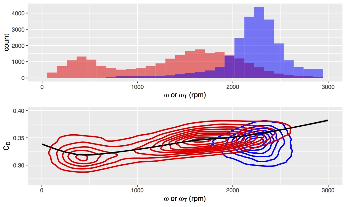
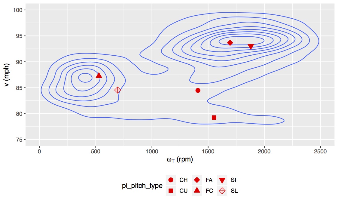
Are there other possible factors that contribute to the variation of CD? Yes, there are two other physical factors that contribute to the variation of CD, the speed v and the spin ω, and these need to be taken into account to determine the true ball-to-ball differences. Actually, it’s a bit more complicated than that, since it is quite likely that CD depends only on the so-called active or transverse spin ωT rather than the total spin ω, where ωT is that part of the spin that contributes to the Magnus effect. While the definitive experiment has not yet been done to confirm this, the data shown in Figure 1 show that of ωT is both broadly distributed and strongly correlated with CD (Pearson correlation coefficient P=0.63). On the other hand, ω is comparatively narrowly distributed and only weakly correlated with CD (P=0.14). The technique for determining ωT from the 9P trajectory is described in the same article that shows how to obtain CD. The distribution of pitches in the ωT–v plane is shown in Figure 2 for 2019, with mean values for each pitch type indicated.
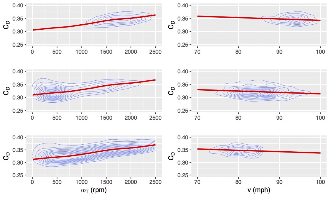
While there are interesting physics reasons — and perhaps even baseball reasons — for exploring the dependence of CD on v and ωT, those dependencies only complicate the present analysis, which is focused on the ball-to-ball variation. Therefore, the approach taken here is to remove these dependencies by fitting CD to v and ωT using a non-parametric general additive model to obtain Cd,fit. An implicit assumption has been made that the dependence of CD on v and ωT is identical for each ball, which differ from each other only by an additive offset. It is the variation of that additive offset that is embodied in σb. Figure 3 compares data with fit for several different pitch types.
Next, several new quantities are defined:
- ∆CD,1 ≡ CD-Cd,fit, which is the difference between the actual and fitted CD and therefore has no dependence on v or ωT. For the 2019 season, ∆CD,1 has approximately zero mean and a standard deviation σ1=0.0166 (reduced from σ=0.0223).
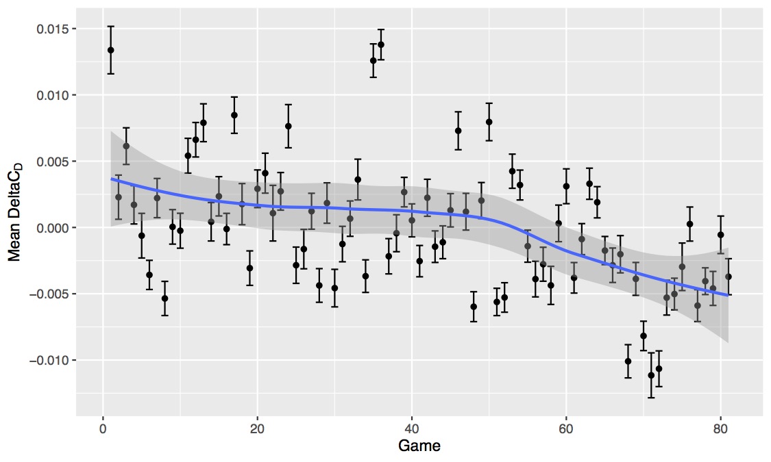
- <∆CD,1>, which is the mean of ∆CD,1 over a single game. Ideally this quantity would not vary from game to game; unfortunately it does, as shown in Figure 4. Indeed, the rms game-to-game variation (0.0048) is more than three times greater than the estimated standard error for each game (≈0.0013), suggesting variation of a non-statistical (and as yet unknown) nature. Perhaps it is due to a change in calibration of the measurement system. Perhaps it is due to unforeseen changes in atmospheric condition, despite the closed stadium. Perhaps it is due to a different collection of baseballs. It is truly not known.
- ∆CD,2 ≡ ∆CD,1 − <∆CD,1>, which removes the game-to-game variation. What remains is the in-game variation, averaged over all games. For 2019, it has zero mean and standard deviation σ2=0.0159. The good news is that the game-to-game variation is small compared to the in-game variation. It is the quantity we will investigate further.
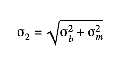
Having removed all the dependence on v and ωT as well as the mysterious game-to- game variation, all the remaining pitch-to-pitch variation in ∆CD,2 should come from the ball-to-ball variation and the measurement noise. That is:
V. Results
The goal is to determine the individual contributions of σb and σm to the total standard deviation σ2 of ∆CD,2. Initially this will be described in detail for 2019 data, then applied to all data 2010-2019. The essential idea of the analysis is as follows. Suppose one takes the difference between ∆CD,2 values of two pitches known to use the same ball. Then the effect of ball variation is removed and the standard deviation of the differences is:
Suppose instead that one takes differences between ∆CD,2 values of two pitches known to use a different ball. The standard deviation of those differences is:
Therefore, by appropriately examining pairs of pitches, one can determine the individual terms σb and σm. As a redundant check, one can calculate the Pearson correlation coefficient P between the pairs, which is expected to be σm2/(σb2 + σm2) and 0 for the same and different balls, respectively.
The results for the standard deviation of differences of ∆CD,2 values between pairs of adjacent pitches and for the correlation P between these pitches is given in Table II for various outcomes of the first pitch in the sequence. The most likely outcome that guarantees that the same ball was used on the subsequent pitch is a called strike. This is true to a lesser extent for a swinging strike or called ball. The most likely way to guarantee that a different ball was used is when the first pitch results in a home run. Unfortunately, there aren’t many such events. Quite often (but not always) a foul ball results in a new ball being used. Probably the most reliable way to guarantee a different ball is to choose a second pitch that is 10 removed in the sequence from the first pitch. These possibilities are all given in the table. Choosing “called strike” and “10 removed” as the two most likely possibilities for same and different ball, respectively, we find that σm and σb are essentially identical and about equal to 0.011-0.012, a result also obtainable from the correlation P ≈ 0.5 for called strikes.
TABLE II: Standard deviation of differences of ∆CD,2 values between pairs of adjacent pitches for various outcomes of the first pitch in the sequence. The number of each category of pairs and the pairwise Pearson correlation coefficient P are also given. The last row considers two pitches separated by ten in the sequence, independent of outcome.
| Outcome | Number | Standard Deviation | P |
|---|---|---|---|
| Called Strike | 4,042 | 0.0168 | 0.525 |
| Swinging Strike | 2,916 | 0.0167 | 0.487 |
| Called Ball | 3,700 | 0.0177 | 0.440 |
| Foul Ball | 3,526 | 0.0220 | 0.097 |
| Home Run | 342 | 0.0216 | 0.071 |
| +10 | 2,376 | 0.0226 | 0.045 |
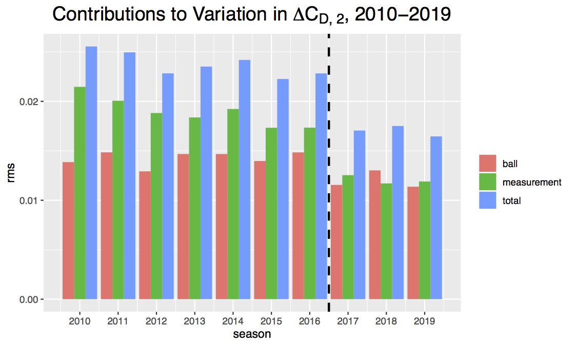
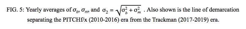
Having developed this technique for the 2019 season, we now apply it to all seasons, 2010-2019. The results are summarized in Figure 5. One clear-cut result is that the measurement precision σm, while relatively constant within each era, is markedly smaller with Trackman (mean=0.012) than with PITCHf/x (mean=0.019). There is smaller difference in the ball-to-ball variation σb, being 0.012 for Trackman and 0.014 for PITCHf/x. Based on a recent analysis, this variation in CD would result in a five-foot variation in distance for a fly ball hit at 100 mph and the optimum launch angle. Except for the small jump between eras, there is no obvious trend in σb. In particular, the data do not support the drag coefficient of the ball being significantly more uniform in the past few years than earlier.
There is one “fly-in-the-ointment” in our analysis. Namely, when two pitches utilize a different ball, then the expectation is that the corresponding values of ∆CD,2 should be uncorrelated; i.e., the Pearson correlation coefficient P should be zero. Table II shows that it is significantly smaller than that obtained when the two pitches utilize the same ball but still not zero for both home runs (with a small data sample) and pitches differing in sequence by 10. Despite much effort, we still do not understand this puzzle. We will leave it for another day.
VI. Summary
In this article, we have discussed the drag on a baseball and what it depends on, including the drag coefficient CD. We have discussed the determination of CD from Statcast pitch-tracking data and have provided the first quantitative comparison between exact CD values determined from the full trajectory and approximate CD values determined from the 9P parametrization of the trajectory. We have discussed the factors leading to variation of pitch-to-pitch CD and have shown how to remove the dependence of CD on the physical factors of ωT and v. We have shown that the remaining variation of CD, namely that due to random measurement noise and ball-to-ball variation, can be separately determined. We find that these two contributions were roughly equal during the Statcast era. Moreover, we find no evidence that the ball-to-ball variation has changed significantly over the period 2010-2019.
Alan Nathan is professor emeritus of physics at the University of Illinois. Visit him at his website, The Physics of Baseball, and follow him on Twitter @pobguy. Charlie Young is a recent graduate of the University of Illinois, Urbana-Champaign, receiving a BS in Computer Science and Astronomy, with a double major in Statistics. He worked alongside Dr. Alan Nathan for the majority of his time at Illinois, and also spent three years as Director of Analytics for the Illinois baseball team. He now works as a Quantitative Developer for the Houston Astros.
Congratulations on getting published here, Charlie!