A New Way to Look at Sample Size

Jonah Pemstein and Sean Dolinar co-authored this article.

Due to the math-intensive nature of this research, we have included a supplemental post focused entirely on the math. It will be referenced throughout this post; detailed information and discussion about the research can be found there.

INTRODUCTION

“Small sample size” is a phrase often used throughout the baseball season when analysts and fans alike discuss player’s statistics. Every fan, to some extent, has an idea of what a small sample size is, even if they don’t know it by name: a player who goes 2-for-4 in a game is not a .500 hitter; a reliever who hasn’t allowed a run by April 10 is not a zero-ERA pitcher. Knowing what small sample size means is easy. The question is, though, when do samples stop becoming small and start becoming useful and meaningful?

This question has been researched before — notably by Russell Carleton, Derek Carty and Harry Pavlidis. Each of them used similar methods of finding reliability to achieve a point of stability.

Our aim in this project is to extend the understanding of reliability and show a more complete picture of how additional plate appearances affect the reliability value of everyday stats for both batters and pitchers. We want to reinforce the idea that reliability is a spectrum, not a single point. There is no single point at which you can say a stat has stabilized. We also want to use the concept of reliability to regress toward the mean and to make confidence bands that give a better idea of a player’s true talent. (Throughout this project we define true talent as the actual talent level — not the value they provide adjusted to park, competition, etc.)

We used a similar approach as Carleton did in his latest reliability study: Cronbach’s alpha. There are, however, differences in our sampling structure, which we explain in more detail in the math post.

METHOD

Sampling

We used a data set that is also similar to Carleton’s most recent studies — Retrosheet data — but we used more recent data from a shorter time frame (2009 to 2014). We also removed intentional walks, bunts and non-batting events such as stolen bases.

From there, we broke the data into different player-seasons instead of just players: 2012 Mike Trout, for example, is different from 2013 Mike Trout. We then used these player-seasons to define samples for a given number of plate appearances (PA), at-bats (AB) or balls in play (BIP). So for 10 PA, we took 10 random plate appearances from each player-season with at least 10 PA; for 600 PA, we took 600 random plate appearances from each player-season with at least 600 PA. As you can imagine, the 10-PA sample has many more player-seasons than the 600-PA sample. Since we used player seasons, we maxed out our sampling at 600 PA, 500 AB and 400 BIP. For anything beyond those limits, the sample size became too small, and results become erratic.

We chose this sampling structure because we think this best represented the general question of the stats’ reliability. The most recent, smaller data set mitigated a bias we found associated with Major League Baseball’s changing run environment. We make no assumptions about a player’s talent levels being the same across years, so we separated each season for each player. This also allows for the comparison of players across years. We will detail the implications and effects of sampling in a future article.

Cronbach’s alpha

There are many different methods to measure reliability, which is mathematically related to correlation but is a different construct with different assumptions. We chose Cronbach’s alpha because it provides a good framework to measure the reliability of a full sample of plate appearances. Given the nature of the data — different parks, pitchers, time of year, etc. — there was no obvious single way to split the data. We used a method that split it in as many ways as possible. Once again, you can read more about Cronbach’s alpha and reliability in the math post.

Cronbach’s alpha’s calculation gives a value — alpha — that is a measurement of the reliability. The value represents the proportion of true-talent variance to the observed variance.

This is not the same as r, r-squared or linear regression.

RESULTS

Alpha

Below is a data visualization of various batting stats’ reliability as it relates to the number of PA/AB/BIP. The lines represent the measured reliability at each 10-PA/AB/BIP increment for each stat. To calculate regression toward the mean and the associated confidence band, enter the stat’s value into the red box and select the appropriate confidence level. Then scroll across the line for the results of the calculation for each PA/AB/BIP increment.

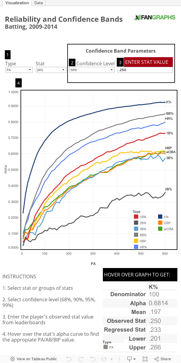
The reliability of each stat increases when the number of PA/AB/BIP increases, and the curve increases at a slower rate as the value gets closer to 1.0. One of the goals of this project is to demonstrate how the reliability of stats changes with number of PA. Most importantly, there is no single point at which a stat becomes stable — every additional PA/AB/BIP simply increases the reliability. Even with a low reliability, there is information within the stat; it just has more noise than a stat with a high reliability.

Regression to the Mean & Confidence Bands

Reliability values are useful for comparison between different stats, but they don’t address the uncertainty of that stat in tangible terms. In other words, it doesn’t give you a likely point or range for the player’s actual skill. Regression to the mean and confidence bands allow us to estimate a floor and ceiling for this uncertainty.

This diagram demonstrates how to regress to the mean and create confidence bands from that regressed stat. Since we are estimating true talent from an observed stat, the first step will be to regress the stat to the mean. If a stat has a low reliability, the sample’s average is a better estimation of the true talent. A high reliability means the stat contains more true-talent information, and that it’s regressed much less toward the mean. Reliability provides an empirical method to regress toward the means in a manner similar to the mathematical approach outline in the appendix of Tango’s The Book (more on that in the math part).

The second part uses the sample’s total standard deviation to estimate the uncertainty and the upper and lower bounds. The higher the standard deviation, the wider the confidence band. (These confidence bands are not the same as the binomial standard error.)

DISCUSSION

All of the previous reliability studies and this one are based in math typically used for test evaluation — where researchers are trying to gauge how well the test is constructed. The basic idea is there is a true score (or in our case talent level), error (or noise) and an observed score (or observed stat).

What reliability attempts to measure is the ratio of the true-talent information to observed information. If there isn’t a lot of true information the reliability will be lower; if there is a lot of information the reliability will be higher. The noise term contains almost every factor that could be associated with affecting a plate appearance: pitcher, park factors, weather, injury and so on. The intent of this analysis is to create reliability measurements and confidence bands for everyday stats, which do not contain these adjustments, so we left all our data unadjusted.

Reliability is partly determined by the distribution of skills within the sample. As a result, sampling becomes an important factor in determining reliability. We tried several variations of sampling structure, including the one Carleton used in his most recent study. The results followed similar patterns, but there were some discrepancies due to different pools of players being used. Using a sample restricted to a high minimum number of PA will decrease the standard deviation because players with better statistics get more PA. This weeds out the lower echelon of players. The remaining players are all bunched tighter together. The larger the spread in talent, the higher the reliability; the smaller the spread, the lower the reliability. We discuss this more in the math post.

Conclusion

The most important conclusion to be drawn is there is no single point at which a stat becomes reliable or stable. The alpha reliability data visualization demonstrates that idea, using the reliability measurement to regress the stat to the mean and create confidence bands. The regressed stat and confidence bands are descriptive, rather than predictive, and are not adjusted for park factors, league adjustments, etc. This can provide an estimation of a player’s true-talent level based on how the player has performed. They aren’t intended to be projections.

NOTES: If you are comparing our results with results from Carleton’s analysis, we are reporting the alpha for the entire sample of PA. His previous analysis found a particular number of PA/AB/BIP associated with a certain value for alpha ( .70) and then halved the PA/AB/BIP value. The Cronbach’s alpha calculation finds the reliability coefficient associated with the entire sample, and it does not need to be halved. Our reporting method is critical to regressing toward the mean and calculating confidence bands.

The code we used — plus a .csv file of the results — are available on GitHub.