A New Way to Look at Sample Size: Math Supplement

This article is co-authored by Jonah Pemstein and Sean Dolinar.

For the introductory, less math-y post that explains more about what this project is, click here.

The concept of reliability comes from the classical test theory designed for psychological, research, and educational tests. The classical test theory uses the model of a true score, error (or noise) and observed score. [2]

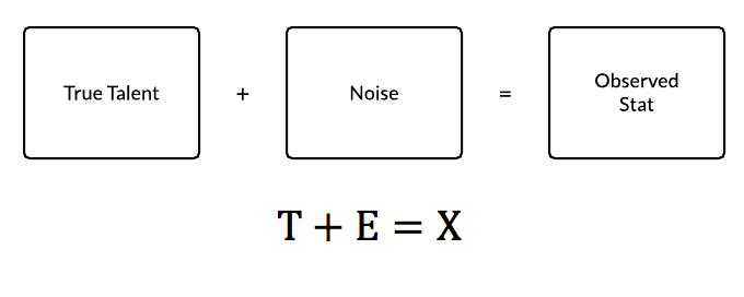
To adapt this to baseball, the true “score” would be the true talent level we are seeking to find, and observed “score” is the actual production of a player. Unfortunately, the true talent level can’t be directly measured. There are several methods to estimate true talent by accounting for different factors. This is, to an extent, what projection systems try to do. For our purposes we are defining the true talent level as the actual talent level and not the value the player provides adjusted to park, competition, etc. The observed score is easy to measure, of course — it’s the recorded outcomes from the games the player in question has played. It’s the stat you see on our leaderboards.

The error term contains everything that can affect cause a discrepancy between the true score and the observed score. It contains almost everything that affects the observed outcome in the stat: weather, pitcher, defenses, park factors, injuries, and so on. This analysis isn’t interested in accounting for those factors but rather measuring the noise those factors in aggregate impart to our observed stat.

ALPHA

Alpha is a coefficient of reliability. Reliability can be generally thought of by its formulation relating the true score’s variance to the observed scored variance. [2, 5]

This can be interpreted as the ratio of variance of the true talent level to the variance of the observed stat score. In this project we refer to this construct of reliability as the reliability coefficient or alpha. We use alpha to specifically refer to the reliability coefficient from Cronbach’s formula. Alpha should not be confused with correlation. Alpha is a measurement associated with an entire test or matrix of scores. Correlation — specifically split-half correlation — is one of many methods to get to the reliability coefficient (and one used previously multiple times in this type of analysis). However, it only describes one half of the the correlated values, because if a split-half correlation (r_ab) is used, the correlation between the two forms represents the reliability of only half of the information, as the test length is cut in half so that one half can be correlated to the other half. The Spearman-Brown Prophecy formula, a formula used to estimate what the reliability of a test will be after changing the length, must be used to get the reliability coefficient (r_XX) for the entire data set. [1]

The correlation between two parallel forms, which is the correlation obtained from two full length tests, shouldn’t be confused with the correlation between the observed stat and the true value, which is given by the square root of the reliability coefficient or alpha. [2]

Cronbach’s alpha represents the average of every possible split-half reliability measurement. This refers to the split-half reliability coefficient, not split-half correlation, which, again, requires the Spearman-Brown formula to obtain the reliability coefficient estimate for the entire sample. [1]

Cronbach’s alpha is, however, only one of several different ways to measure reliability: test-retest, split-half, and parallel forms being other options. As with sampling structure, the choice of reliability measurement is subject to the specific application. Any split-half approach will have a different value depending on how the split of the plate appearances* is executed. [1] Cronbach’s alpha allows us to achieve a unique measurement for reliability for a specific data set. [1]

*Or at bats, or balls in play, depending on the stat we were trying to measure. So, for example, we would use PA for OBP, AB for AVG, and BIP for BABIP. Whenever we say “plate appearances” in this post, know that we mean PA/AB/BIP.

Nearly all previous studies on this topic as it relates to baseball have used either a version of split-half reliability [9, 10] or Cronbach’s alpha*, and the most recent studies use Cronbach’s alpha. [7, 8]

*In Carleton’s most recent work on this, he used the Kuder-Richardson 21 formula, which is the mathematical equivalent of Cronbach’s alpha for binary data. This works fine for data that are binary, but we chose to use Cronbach’s alpha for everything for ease of not having to code for multiple formulas — not everything is binary.

We calculated alpha for 10-PA/AB/BIP increments for K. To calculate it, we set up N x K matrices including each plate appearance in our sample, where K represents the number of plate appearances and N represents the number of players. Each matrix looks like the following table (Player Totals are the sum of the rows):

There are many different ways to formulate Cronbach’s alpha. For the specific application of this project the follow formulation is used [1]:

Where i represents each plate appearance 1 through K, t represents the Player Totals for each player 1 through N, and K is as defined above.

This formula uses the ratio of the variance of each plate appearance among all players (s_i²) and inter-player variance (s_t²). The variance within the PA can be thought of as the noise within the particular stat. The inter-player variance is the variance of the Player Totals column in the example matrix. (It should be noted this variance term is the variance of the sum of the binomial outcomes for each player and not of the sum divided by K.) Subtracting this ratio from 1 yields the relationship for alpha: the ratio of true variance to the observed stat variance.

This formula is helpful in understanding what factors affect the alpha measurement. High variance within the plate appearances and low variance between the players will lead to a low reliability. Since the plate appearances are being treated equally, the variances within will generally be the same for every PA column. But the inter-player variance, on the other hand, changes greatly depending on the stat we are measuring; since more variation among players means a larger alpha, stats such as strikeout percentage (K%) — for which there is a lot of variation in the population of players — will have a higher reliability coefficient than stats such as HBP% (hit by pitch per plate appearance), where the variation is much lower.

The impact of sample variance is best demonstrated by two example data sets. Both were created using a normal distribution of player talent levels centered around a league average of .300, and then a random binomial generator was used to simulate 100 plate appearances. The only parameter that was varied was the standard deviation of the the normal distribution for the player talent levels. The lower variance group were more tightly concentrated around .300, while the high variance group have much more spread.

While the variance within PAs remained more or less the same, the variance among players had a pronounced effect on alpha.

DESIGN

To get our PA matrices for each number of plate appearances (K), we selected a random sample of K plate appearances from each player-season from 2009-2014 with at least K plate appearances. This allows for inclusion of the most players. As K grew, the number of players (N) in the matrix naturally decreased significantly, but this is also representative of the selection bias that occurs during the season as better players get more PAs. Since both the reliability coefficient and the confidence bands are dependent on the sample, it’s important to view any analysis within the context of the parameters of each reliability measurement.

SAMPLING

We tested a few different sampling approaches: Carleton’s original 2000-PA/2000-AB/1000-BIP sampling structure, our K-PA dynamic sampling data set, and our technique using chronological selection of the PA as opposed to randomizing them.

While we noticed some differences, most of the empirical findings are fairly similar. The reliabilities’ relative positions to each other remain rather consistent. The greatest discrepancy we found between different sampling structures was with SLG and ISO, where Carleton’s sampling structure produced lower alpha measures, mostly due to lower inter-player variances.

The graphic above shows on the more dramatic examples of the discrepancy of between different sampling structures. The inter-player variance is lower in Carleton’s 2000-AB (yellow) sampling structure than it is using the K-PA dynamic sampling approach (green and blue). The sample mean also doesn’t change for the 2000-AB, while the dynamic sampling structure’s sample mean gradually rises.

Chronological sampling also reduced the reliability for low numbers of PA because grouping the first PA/AB/BIP in the data set together group many players’ early plate appearances together. Since player talent does vary with age and experience, this most likely contributes to the slightly reduction in reliability.

Finally, the time frame impacts the reliability, because of the dynamic nature of baseball. The run environment has dramatically changed since 2002. Having stats from a high-run environment mixed with stats from a low-run environment creates an inflated inter-player variance.

As mentioned in the introductory post for this project, this reveals that reliability measurements should be done on samples which are specific to the application. We will fully investigate this concept further in a future post and attempt to refine a sampling structure.

REGRESSION TO THE MEAN

One of the uses of reliability is to use the coefficient to determine how much to regress towards the mean. The following equation uses the measured alpha value to determine how much of the observed stat to use versus using the sample mean. As the stat becomes more reliable, it has to be regressed towards the mean less. [6]

The equation is similar to the one outlined by Tango, Litchman & Dolphin [3], except alpha is replaced. In fact, alpha and Tango’s equation have the same basic inputs: variance of the stat and the inter-player variance.

The Book draws conclusions regarding regressing towards the mean that are similar to the ones we discussed in regards to formulation of Cronbach’s alpha:

“If the standard deviation of the population is quite small, one assumes that deviations from this are probably due to random deviations and thus one estimates player abilities very close to the overall averages. On the other hand, if the standard deviation of the population is large, the reverse is true.”

In other words, the inter-player variance has a large effect on regression towards the mean using Tango’s formula. This is the same conclusion we drew from before about inter-player variance’s effect on alpha.

One other difference in our formulation of regression toward the mean is that Tango’s formula uses the league average while we use the sample average. The sample mean refers to the mean of players with K plate appearances, since each reliability coefficient is measured in the context of the players in that sample. With a static sampling structure, the inter-player variance shrinks as more plate appearances are added. We used a dynamic sampling structure, so both the mean and variance change as K grows larger and the size of the player pool shrinks.

CONFIDENCE BANDS

Confidence bands are constructed using the regressed stat as the point estimate. From the point estimate, the standard error of the measurement (SEM) is used to create a lower and upper bound. The SEM uses alpha to determine how of the inter-player standard deviation to include. [6]

The confidence band is constructed by adding and subtracting the SEM multiplied by the appropriate z-score to the regressed stat.

This creates a confidence interval around the regressed stat and not the observed stat. For extreme values, the confidence interval might not contain the observed stat.

CONCLUSION

While the intention of this project wasn’t to find something groundbreaking, we did discover more subtle findings which affect the reliability measurement. As already mentioned, it’s not really possible achieve a universal sampling structure, because reliability is dependent on what you are comparing.

One of the extensions of the issue with sampling is choosing an appropriate time frame. Using more data in this case doesn’t always make alpha more accurate. Including the high-run environment of the early 2000s with the low-run environment of the 2010s creates more inter-player variance, which will artificially inflate the reliability numbers, and mixes in data from a different run environment, which we do not want.

The findings of this project are by no means a panacea for determining when particular stats are good to use, but we think they certainly help a lot and we hope that they will steer research on this topic in the direction of confidence bands and uncertainty measurements instead of fixed stabilization points. We acknowledge that there are several other approaches that could be used. Even within the reliability-regress to the mean framework, the sampling structure can always be improved and adjustments could be made to correct for park factors, run environment, and league.

The code we used — plus a .csv file of the results — are available on GitHub.

GLOSSARY

K — number of items (PA, AB, BIP).

N — number of subjects (players).

PA/AB/BIP — plate appearances, at bats, and balls in play, the items in a reliability sample. Depending on the denominator of the stat, the PA, AB, and BIP will change. We said simply “plate appearances” many times throughout this post to refer to all of PA, AB, and BIP.

Alpha — Cronbach’s alpha. We are using it for the reliability measurement (or coefficient). Alpha can be interpreted as the proportion of true variance to observed variance.

Observed Stat — the stat found on our leaderboards. What the player actually did.

Regressed Stat — the stat that has been regressed to the mean using the reliability coefficient.

Inter-player variance — the variance among player totals in the PA matrix. (The summed totals are the final column of the matrix in the example we provided above.)

Within-plate appearance variance — the variance within a column. The variance of each column is taken then the variances are summed together.

Random Dynamic Sampling — uses a dynamic sampling draw for all player-seasons with at least K plate appearances, and randomly selects plate appearances from that player-season to be included in the PA matrix.

Chronological Dynamic Sampling — uses dynamic sampling but it draws the player’s first, second, third, etc. PA/AB/BIP in the data set to put into the matrix.

Chronological 2000-PA Sampling — finds a subset of Players which have 2000 PA/AB/BIP in the data set, then chronologically orders the PA/AB/BIP for the matrix. (Carleton used this for his most recent studies with the notable exception of 1000 BIP instead of 2000.)

Sample mean — the average value of a stat for the player contained within a reliability measurement sample.

Sample standard deviation/variance — the standard deviation or variance of the players stats within a reliability measurement sample.

REFERENCES

[1]

Cronbach, Lee J. (September, 1951). Coefficient alpha and the internal structure of tests. Psyschometrika. Vol 16, No: 3.

[2]

Gulliksen, Harold. (1950). Theory of mental tests. Hillsdale, NJ: Lawrence Erlbaum Associates, Inc. [Questia access required]

[3]

Tango, T., Lichtman, M., & Dolphin, A. (2007). The book: Playing the percentages in baseball. Dulles, VA: Potomac Books, Inc.

[4]

Cronbach’s alpha. (n.d.). In Wikipedia. Retrieved June 16, 2015 from https://en.wikipedia.org/wiki/Cronbach%27s_alpha

[5]

Reliability (psychometrics). (n.d.). In Wikipedia. Retrieved June 16, 2015 from https://en.wikipedia.org/wiki/Reliability_(psychometrics)

[6]
Weir, Joseph P. (Feb 1, 2005). Quantifying test-retest reliability using the intraclass correlation coefficient and the SEM. Journal of Strength and Conditioning Research, 19(1), 231-240.

[7]
Carleton, Russell A. (July 16, 2012). Baseball therapy: It’s a small sample size after all. Baseball Prospectus. Retrieved from http://www.baseballprospectus.com/article.php?articleid=17659.

[8]
Carleton, Russell A. (May 9, 2013). Baseball therapy: Should i worry about my favorite pitcher?. Baseball Prospectus. Retrieved from http://www.baseballprospectus.com/article.php?articleid=20516.

[9]
Carty, Derek. (June 20, 2011). Resident fantasy genius: When pitchers’ stats stabilize. Baseball Prospectus. Retrieved from http://www.baseballprospectus.com/article.php?articleid=14293.

[10]
Carty, Derek. (June 13, 2011). Resident fantasy genius: When hitters’ stats stabilize. Baseball Prospectus. Retrieved from http://www.baseballprospectus.com/a/14215.