Estimating ERA: A Simulated Approach

ERA, probably the single most cited reference for evaluating the performance of a pitcher, comes with a lot of problems. Neil does a good job outlining why in this FanGraphs Library entry. Over the last decade, plenty of research has cast a light on the variables within ERA that often have very little to do with the pitcher himself.

But what is the best way to use fielding-independent stats to estimate ERA? FIP is probably the most popular metric of this ilk, using only strikeouts, walks, hit batters, and home runs to create a linear equation that can be scaled to look like an expected ERA. Then there’s xFIP, which is based off the idea that pitchers have very little control over their HR/FB rate; to account for this, it estimates the amount of home runs that a pitcher should have allowed by multiplying their fly balls allowed by the league average HR/FB rate.

For many people, however, these are too simple. FIP more or less ignores all balls in play completely; xFIP treats all fly balls equally. Neither one correctly accounts for the effects that any ball in play can have; we know that the wOBA on line drives is much higher than the wOBA on pop ups, but we don’t see that reflected in many ERA estimators. The estimators we use also are fully linear, and may break down at the extreme ends; FIP tells us that a pitcher who strikes out every batter should have an ERA around -5.70, which is, well you know, not going to happen.

This is where simulations can help. I’m a big fan of simulations and think that they can be tremendously powerful and accurate tools when used correctly. So what I have done is created a Markov-esque* simulation to estimate a pitcher’s ERA with the following inputs: K%, BB% (which I will refer to a lot throughout this article, and every time will mean BB+HBP%, since walks and hit batsmen are for our purposes the same thing), and HR% (these three are the FIP inputs); and GB%, FB%, LD%, and IFFB%. The goal is to produce a more accurate ERA estimator that still only takes into account the pitcher’s fielding-independent stats.

*I say Markov-esque because in the technical definition of a Markov chain, each state is a result only of the state that preceded it. This is not really the case in this simulator, as you will see.

Here’s how I did this. First, I assigned each of the 7 inputs a range between 0 and 1. For example, if the pitcher had a 20% K%, an 8% BB%, and a 2% HR%, this is what those ranges would look like:

0 – 0.2: K
0.2 – 0.28: BB
0.28 – 0.3: HR

And then if they had a 50% GB%, a 35% FB%, a 15% LD%, and a 10% IFFB%, here’s what those ranges would look like:

0.3 – 0.65: GB
0.65 – 0.8705: OFFB
0.8705 – 0.895: IFFB
0.895 – 1: LD

These were calculated using the fact that GB%, FB%, and LD% are grounders, fly balls, and line drives per ball in play, not per batter, like K%, BB%, and HR%. So for our made-up pitcher, who allowed a ball in play 70% of the time, each of his GB%, FB%, and LD% had to be multiplied by 0.7. Then IFFB (infield fly balls — pop ups) were separated from OFFB (outfield fly balls) by multiplying FB% by IFFB% and 1-IFFB%, respectively. (Remember that IFFB% is not pop ups per ball in play, but rather pop ups per fly ball. So GB%+FB%+LD%+IFFB% doesn’t equal 1, GB%+FB%+LD% does.)

Note: I realize that home runs can be considered balls in play, and are included in fly ball rates. So when inputting numbers, you’ll have to use the fly ball rate that doesn’t include home runs. Don’t worry about calculating that for yourself; I’ve done it for you.

Then I defined three variables: the outs, the runs that had scored, and the runners. The beginning of the simulation, naturally, is a situation where there are no outs, no runs in, and no runners on base. From there, I generated a random number between 0 and 1. This number would fall into the range of one of the outcomes.

Then it got interesting. If the random number fell within the range for a strikeout, walk, or home run, what happened next was simple: a strikeout added one out to the current number of outs, and if that made 3 outs, the bases reset. A walk added a runner to the next available base or added one run if the bases were loaded. A home run cleared the bases and added the appropriate amount of runs. If the random number fell within the range for one of the batted balls, things were considerably more complex. Here are the outcome distributions for each of the batted ball types (home runs excluded):

Ball in play	Out	1B	2B	3B
OFFB	86.0%	4.2%	8.5%	1.4%
GB	76.5%	21.7%	1.7%	0.1%
LD	32.2%	51.6%	14.9%	1.3%
IFFB	98.9%	0.7%	0.4%	0.0%

So if the first random number dictated some sort of ball in play, a second random number was used to determine what type of hit the ball in play would be, which would of course depend on what type of batted ball it was in the first place. But wait, there’s more! How do the runners advance on different types of batted balls? Well, as one would expect, runners advance bases differently on singles than they do on doubles, but they also advance differently on, say, ground ball doubles than they do on fly ball doubles. So I had to find out how runners move on the basepaths for different types of balls in play and different types of hits. Here’s what I found:

Hit Type	BIP	xxx -> xxx	xxx -> 1xx	xxx -> 12x	xxx -> 123	xxx -> 1×3	xxx -> x2x	xxx -> x23	xxx -> xx3
1B	FB	3.5%	95.2%				1.3%		0.1%
1B	GB	0.4%	98.4%				1.2%		0.1%
1B	LD	0.9%	98.5%				0.5%		0.1%
1B	PU	2.7%	93.3%				2.7%		1.3%
2B	FB	0.9%					98.5%		0.6%
2B	GB	0.4%					98.7%		0.9%
2B	LD	0.5%					99.0%		0.6%
2B	PU	1.7%					98.3%
3B	FB	1.4%							98.6%
3B	GB	2.1%							97.9%
3B	LD	0.9%							99.1%
3B	PU								100.0%
O	FB	98.5%	0.1%				1.4%
O	GB	97.1%	2.5%				0.4%
O	LD	97.7%	0.6%				1.7%		0.1%
O	PU	99.6%	0.2%				0.2%

Hit Type	BIP	1xx -> xxx	1xx -> 1xx	1xx -> 12x	1xx -> 123	1xx -> 1×3	1xx -> x2x	1xx -> x23	1xx -> xx3
1B	FB	0.1%	2.8%	57.4%		35.0%	1.4%	1.8%	1.5%
1B	GB	0.1%	0.9%	72.2%		25.0%	0.4%	1.2%	0.3%
1B	LD	0.1%	0.9%	69.1%		27.0%	0.7%	1.2%	0.9%
1B	PU		11.1%	58.3%		27.8%			2.8%
2B	FB	1.8%					51.7%	42.0%	4.5%
2B	GB	0.9%					25.0%	70.8%	3.3%
2B	LD	1.3%					35.8%	58.6%	4.4%
2B	PU						28.6%	71.4%
3B	FB	1.0%							99.0%
3B	GB	5.9%							94.1%
3B	LD	3.1%							97.0%
3B	PU
O	FB	1.0%	96.3%	0.1%		0.1%	1.3%	1.2%
O	GB	30.2%	52.0%	2.8%		0.9%	13.8%	0.3%	0.1%
O	LD	11.0%	85.3%	0.5%		0.2%	1.3%	1.6%	0.2%
O	PU	0.5%	99.2%	0.1%		0.2%	0.1%

Hit Type	BIP	12x -> xxx	12x -> 1xx	12x -> 12x	12x -> 123	12x -> 1×3	12x -> x2x	12x -> x23	12x -> xx3
1B	FB		1.8%	22.2%	41.0%	26.4%	2.1%	4.9%	1.5%
1B	GB	0.2%	1.3%	36.0%	36.3%	20.3%	0.7%	4.5%	0.8%
1B	LD	0.2%	2.2%	36.7%	28.3%	25.1%	1.4%	5.1%	1.0%
1B	PU				58.3%	33.3%	8.3%
2B	FB	1.4%					55.4%	39.2%	4.1%
2B	GB	1.8%					29.6%	66.3%	2.4%
2B	LD	1.3%					41.6%	54.2%	2.9%
2B	PU						50.0%	50.0%
3B	FB	2.4%							97.6%
3B	GB								100.0%
3B	LD	3.3%							96.7%
3B	PU
O	FB	0.1%	0.3%	80.7%	0.1%	14.8%	0.3%	3.5%	0.2%
O	GB	0.1%	1.9%	46.4%	2.2%	13.8%	16.9%	10.6%	8.1%
O	LD	0.1%	9.2%	81.5%	0.2%	3.6%	3.2%	2.2%	0.2%
O	PU		0.1%	99.3%	0.1%	0.2%		0.1%	0.1%

Hit Type	BIP	123 -> xxx	123 -> 1xx	123 -> 12x	123 -> 123	123 -> 1×3	123 -> x2x	123 -> x23	123 -> xx3
1B	FB		0.8%	18.0%	59.0%	16.4%		4.9%	0.8%
1B	GB		1.9%	32.4%	39.7%	19.0%	0.2%	5.7%	1.1%
1B	LD		1.4%	31.8%	35.7%	24.5%	1.3%	4.4%	0.8%
1B	PU				66.7%	33.3%
2B	FB	0.6%					49.7%	47.3%	2.4%
2B	GB						38.3%	60.0%	1.7%
2B	LD	1.0%					38.8%	56.7%	3.4%
2B	PU
3B	FB	2.9%							97.1%
3B	GB								100.0%
3B	LD	2.9%							97.1%
3B	PU
O	FB		0.7%	20.1%	57.1%	15.2%	0.5%	6.3%	0.2%
O	GB		0.7%	4.0%	56.4%	11.6%	0.6%	22.3%	4.4%
O	LD		0.5%	20.6%	61.0%	10.6%		7.0%	0.3%
O	PU			0.7%	98.9%	0.2%		0.2%

Hit Type	BIP	1×3 -> xxx	1×3 -> 1xx	1×3 -> 12x	1×3 -> 123	1×3 -> 1×3	1×3 -> x2x	1×3 -> x23	1×3 -> xx3
1B	FB		3.2%	54.5%		38.5%	1.3%	1.9%	0.6%
1B	GB		1.2%	74.6%	0.3%	21.4%	0.4%	1.5%	0.6%
1B	LD		1.4%	69.1%	0.1%	26.6%	1.0%	1.5%	0.4%
1B	PU			57.1%		42.9%
2B	FB	0.4%					54.3%	42.8%	2.5%
2B	GB	1.3%					28.8%	65.0%	5.0%
2B	LD	1.4%					40.1%	55.6%	3.0%
2B	PU
3B	FB								100.0%
3B	GB	14.3%							85.7%
3B	LD								100.0%
3B	PU								100.0%
O	FB	0.8%	33.8%	0.3%		56.9%	5.3%	2.4%	0.5%
O	GB	5.5%	10.6%	7.3%	0.2%	49.6%	6.8%	3.2%	16.8%
O	LD	0.5%	26.8%	0.5%		62.0%	1.8%	2.1%	6.4%
O	PU		1.3%			97.6%	0.6%	0.2%	0.3%

Hit Type	BIP	x2x -> xxx	x2x -> 1xx	x2x -> 12x	x2x -> 123	x2x -> 1×3	x2x -> x2x	x2x -> x23	x2x -> xx3
1B	FB	3.9%	53.3%	5.8%		31.5%	4.9%	0.7%
1B	GB	1.5%	46.7%	4.0%		38.7%	8.2%	0.5%	0.5%
1B	LD	3.1%	54.3%	0.7%		30.2%	10.1%	0.7%	1.1%
1B	PU		33.3%	22.2%		44.4%
2B	FB	0.9%					92.3%	6.0%	0.8%
2B	GB	0.5%					97.8%	0.9%	0.9%
2B	LD	0.3%					98.4%	0.8%	0.5%
2B	PU						33.3%	66.7%
3B	FB	1.9%							98.2%
3B	GB	8.3%							91.7%
3B	LD	2.0%							98.0%
3B	PU
O	FB	0.8%	0.1%	0.1%		0.1%	81.1%	0.1%	17.9%
O	GB	0.2%	3.0%	0.6%		1.9%	58.7%	0.1%	35.5%
O	LD	5.5%	0.5%	0.1%		0.3%	87.6%	0.1%	5.9%
O	PU	0.2%	0.3%			0.2%	98.7%		0.6%

Hit Type	BIP	x23 -> xxx	x23 -> 1xx	x23 -> 12x	x23 -> 123	x23 -> 1×3	x23 -> x2x	x23 -> x23	x23 -> xx3
1B	FB	3.3%	38.5%	6.6%	1.1%	44.0%	5.5%	1.1%
1B	GB	1.1%	46.7%	3.3%	1.9%	40.2%	5.9%		1.0%
1B	LD	1.8%	51.1%	0.4%	0.3%	36.9%	7.9%	0.9%	0.9%
1B	PU		50.0%			50.0%
2B	FB	0.7%					92.7%	6.0%	0.7%
2B	GB						100.0%
2B	LD	0.5%					98.6%	0.5%	0.5%
2B	PU
3B	FB								100.0%
3B	GB								100.0%
3B	LD	4.8%							95.2%
3B	PU
O	FB	0.7%	0.1%	0.1%		0.3%	20.8%	56.1%	21.9%
O	GB		1.6%	2.7%	0.3%	7.9%	7.4%	59.5%	20.5%
O	LD	0.2%	0.2%	0.2%		0.7%	20.1%	70.1%	8.6%
O	PU		0.3%	0.3%			0.3%	98.1%	1.1%

Hit Type	BIP	xx3 -> xxx	xx3 -> 1xx	xx3 -> 12x	xx3 -> 123	xx3 -> 1×3	xx3 -> x2x	xx3 -> x23	xx3 -> xx3
1B	FB	4.7%	92.2%			0.8%	2.3%
1B	GB	0.3%	96.5%			1.8%	1.4%
1B	LD	1.0%	98.1%			0.2%	0.7%
1B	PU		75.0%				25.0%
2B	FB	1.8%					98.2%
2B	GB						100.0%
2B	LD	0.3%					99.0%		0.7%
2B	PU						100.0%
3B	FB	5.0%							95.0%
3B	GB								100.0%
3B	LD								100.0%
3B	PU
O	FB	33.8%	0.1%			0.1%	1.1%		64.9%
O	GB	15.7%	7.6%			0.4%	1.7%	0.1%	74.6%
O	LD	25.1%	0.3%			0.1%	2.0%		72.4%
O	PU	0.9%	0.6%				0.2%		98.3%

(xxx = bases empty, 123 = bases loaded, x2x = runner on second, etc.). If you’re interested in those numbers, here is the download link for the Excel file, and here is the dowload link for the .csv file.

Anyways, I would generate a third random number to determine how the runners advanced. Say the first two random numbers dictated a single on a ground ball, and there were runners on first and third. If you look at the table above, you’ll see that in that situation and with a ground ball single, the baserunner situation changes to first and second about 75% of the time, to first and third (which isn’t really a change) about 21.5% of the time, and to other various things about 3.5% of the time. So if my third random number was below .75, the base state would change to first and second; if the number was between .75 and .965, the base state wouldn’t change; and so on. (Actually, to preserve my sanity and to avoid having to monotonously type so many things into a program, I rounded a little and removed events that almost never happened; here, I went with a 77-23 split and eliminated all the other small possibilities because they were so rare anyways.)

And of course, a run scored there. So I would add a run to the amount of runs that had scored. But sometimes yet more random numbers were needed — in cases where it was ambiguous whether people who got taken off the basepaths scored or got tagged/forced out. Another example: On fly ball outs where the base-state goes from “xx3” to “xxx”, it’s clear that a runner tried to tag up and score on a sacrifice fly. But how do we decide if the runner made it or not? I found the proportion of times where there was one run scored on the play and one out, and the proportion of times where there were no runs scored and two outs. (In this case, the split was actually a surprising 97.15% success rate for the runner tagging up — in a sample of 738 tries!) I then used my fourth random number to determine how many runs scored and how many outs were made on each play where it may have been unclear.

That’s pretty much how my simulator works. It runs until the desired amount of innings pitched has gone by and then gives an ERA, which is just the number of runs that scored divided by the innings times nine. But you’d think that with all the randomness that goes into the simulation, it has to be run many, many times in order to get a meaningful and stable result. And that’s precisely the point.

In a normal season, pitchers nowadays will get a maximum of roughly 250 innings pitched, and almost always fewer, especially if they are relievers. That’s part of what makes ERA so volatile; there’s so much randomness and luck that goes on in that relatively small amount of innings. This simulator, however, can simulate hundreds of thousands of innings in just seconds. That is enough to strip almost all of the luck out of the result, because eventually all of the random numbers will average out, something which they do not have time to do in a pitcher’s season.

Of course, this is all resting on one assumption, and that’s that pitchers don’t have control over their balls in play past what type they are. This we know not to be entirely true, and it really doesn’t make any sense, either: if pitchers can control the kind of balls that get put into play (which they can, something that this nifty tool shows us), who’s to say that they can’t control the quality of contact, at least to some extent? But until we find a way to quantify that, we’re going to have to go with what we know. My next article is going to discuss how to figure out how much pitchers can control what happens on their balls in play, and from there I will try to incorporate that into this model.

Additionally, this method entirely ignores the instability of HR/FB rate, and is more like FIP in that way — it doesn’t think about home runs being somewhat luck-driven, and instead assumes that the pitcher has complete control over them. Maybe in the future I’ll create another version of this simulator that is more similar to xFIP.

Ok, finally: here’s the Python script (in Python 2.7) for you to be able to run the simulator. If you don’t know how to use that, you can copy and paste the code into something like Evaluzio, but just know that that’s a lot slower. (Hit the “Try it now” button towards the right on the Evaluzio homepage to get to the code editor.)

If you want to be able to download the script but you don’t know how: download Python 2.7.9 (or whatever the latest version starting with 2.7 is) from here. Open Idle (which was downloaded as part of the Python download) and create a new window (command/control + N, depending on if you’re using Mac/Windows). Copy the Python file above and paste it into that window. Run the script (F5 button) and put in the inputs. It works pretty fast — like, simulating 100,000 innings in under 2 seconds fast.

And here is a table of pitchers with each of the stats needed for this simulator:

When you’re running the simulation, don’t input the player’s normal batted ball profile, because that includes home runs — this simulation regards home runs as totally separate from other fly balls, which is reflected in the table above. Also, I would advise running at least 100,000 innings for each simulation — that way, it will be fairly stable without taking too much time.

And as a reference, here is a table of pitchers with at least 340 total batters faced and what the simulator — do I need a name for this? I’ll call it SERA, for Simulated ERA — says their ERA should be. Each one has had 500,000 innings simulated:

Rank	Name	SERA	FIP	ERA
1	Dellin Betances	1.78	1.64	1.40
2	Clayton Kershaw	1.97	1.81	1.77
3	Chris Sale	2.44	2.57	2.17
4	Jake Arrieta	2.46	2.26	2.53
5	Carlos Carrasco	2.58	2.44	2.55
6	Corey Kluber	2.59	2.35	2.44
7	Felix Hernandez	2.60	2.56	2.14
8	Garrett Richards	2.66	2.60	2.61
9	Anibal Sanchez	2.75	2.71	3.43
10	Marcus Stroman	2.83	2.84	3.65
11	Jon Lester	2.86	2.80	2.46
12	Yusmeiro Petit	2.93	2.78	3.69
13	Alex Cobb	2.94	3.23	2.87
14	Gio Gonzalez	2.97	3.03	3.57
15	Jordan Zimmermann	2.97	2.68	2.66
16	Jacob deGrom	2.98	2.67	2.69
17	David Price	2.99	2.78	3.26
18	Hyun-Jin Ryu	3.00	2.62	3.38
19	Phil Hughes	3.02	2.65	3.52
20	Carlos Villanueva	3.04	3.13	4.64
21	Yu Darvish	3.05	2.84	3.06
22	Max Scherzer	3.06	2.85	3.15
23	Dallas Keuchel	3.08	3.21	2.93
24	Gerrit Cole	3.09	3.23	3.65
25	Jose Quintana	3.09	2.81	3.32
26	Madison Bumgarner	3.12	3.05	2.98
27	Jeff Samardzija	3.18	3.20	2.99
28	Johnny Cueto	3.20	3.30	2.25
29	Carlos Martinez	3.22	3.18	4.03
30	Lance Lynn	3.26	3.35	2.74
31	Adam Wainwright	3.28	2.88	2.38
32	Cliff Lee	3.29	2.96	3.65
33	Stephen Strasburg	3.29	2.94	3.14
34	Alex Wood	3.30	3.25	2.78
35	Cole Hamels	3.30	3.07	2.46
36	Zack Greinke	3.31	2.97	2.71
37	Andrew Cashner	3.31	3.09	2.55
38	Scott Kazmir	3.32	3.35	3.55
39	Michael Wacha	3.32	3.17	3.20
40	Tyson Ross	3.35	3.24	2.81
41	Matt Shoemaker	3.37	3.26	3.04
42	Zack Wheeler	3.43	3.55	3.54
43	Sonny Gray	3.43	3.46	3.08
44	Collin McHugh	3.44	3.11	2.73
45	Tyler Skaggs	3.46	3.55	4.30
46	Ian Kennedy	3.48	3.21	3.63
47	Tanner Roark	3.51	3.47	2.85
48	Masahiro Tanaka	3.54	3.04	2.77
49	Danny Duffy	3.54	3.83	2.53
50	Hisashi Iwakuma	3.55	3.25	3.52
51	Vance Worley	3.55	3.44	2.85
52	Chris Archer	3.55	3.39	3.33
53	Francisco Liriano	3.57	3.59	3.38
54	Brett Oberholtzer	3.58	3.56	4.39
55	Zach McAllister	3.59	3.45	5.23
56	James Shields	3.60	3.59	3.21
57	Nathan Eovaldi	3.61	3.37	4.37
58	Julio Teheran	3.61	3.49	2.89
59	Matt Garza	3.62	3.54	3.64
60	Odrisamer Despaigne	3.63	3.74	3.36
61	Tom Koehler	3.66	3.84	3.81
62	Justin Verlander	3.66	3.74	4.54
63	Drew Hutchison	3.66	3.85	4.48
64	Doug Fister	3.67	3.93	2.41
65	Charlie Morton	3.68	3.72	3.72
66	Hiroki Kuroda	3.69	3.60	3.71
67	Danny Salazar	3.70	3.52	4.25
68	Carlos Torres	3.71	3.86	3.06
69	Drew Smyly	3.73	3.77	3.24
70	Tim Hudson	3.75	3.54	3.57
71	Yordano Ventura	3.76	3.60	3.20
72	Mat Latos	3.78	3.65	3.25
73	Jake Odorizzi	3.78	3.75	4.13
74	Kyle Gibson	3.79	3.80	4.47
75	Jenrry Mejia	3.80	3.73	3.65
76	Shane Greene	3.80	3.73	3.78
77	Edinson Volquez	3.80	4.15	3.04
78	Kevin Gausman	3.81	3.41	3.57
79	Anthony Swarzak	3.82	3.77	4.60
80	Bartolo Colon	3.82	3.57	4.09
81	Clay Buchholz	3.84	4.01	5.34
82	Dan Otero	3.86	3.28	2.28
83	Henderson Alvarez	3.86	3.58	2.65
84	Tyler Matzek	3.86	3.78	4.05
85	Jarred Cosart	3.87	3.77	3.69
86	Kyle Lohse	3.87	3.95	3.54
87	T.J. House	3.88	3.69	3.35
88	Ervin Santana	3.88	3.39	3.95
89	Aaron Harang	3.92	3.57	3.57
90	Mark Buehrle	3.93	3.66	3.39
91	Mike Leake	3.93	3.88	3.70
92	Rick Porcello	3.94	3.67	3.43
93	Homer Bailey	3.97	3.93	3.71
94	Jake Peavy	3.99	4.11	3.73
95	Jon Niese	4.00	3.67	3.40
96	Brandon McCarthy	4.00	3.55	4.05
97	John Lackey	4.00	3.78	3.82
98	Roenis Elias	4.01	4.03	3.85
99	Jered Weaver	4.03	4.19	3.59
100	Wily Peralta	4.04	4.11	3.53
101	Josh Collmenter	4.05	3.87	3.46
102	Chris Tillman	4.07	4.01	3.34
103	Daisuke Matsuzaka	4.08	4.21	3.89
104	Jason Hammel	4.08	3.92	3.47
105	Wei-Yin Chen	4.09	3.89	3.54
106	David Buchanan	4.10	4.27	3.75
107	Dan Haren	4.10	4.09	4.02
108	A.J. Burnett	4.11	4.14	4.59
109	Jason Vargas	4.11	3.84	3.71
110	Yovani Gallardo	4.12	3.94	3.51
111	Hector Santiago	4.13	4.29	3.75
112	Jesse Chavez	4.13	3.89	3.45
113	Brad Hand	4.16	4.20	4.38
114	Jorge de la Rosa	4.16	4.34	4.10
115	Bud Norris	4.17	4.22	3.65
116	R.A. Dickey	4.17	4.32	3.71
117	Trevor Bauer	4.19	4.01	4.18
118	Ryan Vogelsong	4.21	3.85	4.00
119	Wade Miley	4.23	3.98	4.34
120	Samuel Deduno	4.23	4.31	4.47
121	Cesar Ramos	4.23	4.25	3.70
122	Jeremy Guthrie	4.24	4.32	4.13
123	David Hale	4.24	4.31	3.30
124	Justin Masterson	4.29	4.50	5.88
125	Josh Beckett	4.30	4.33	2.88
126	Trevor Cahill	4.36	3.89	5.61
127	Scott Feldman	4.36	4.11	3.74
128	J.A. Happ	4.37	4.27	4.22
129	Bronson Arroyo	4.38	4.32	4.08
130	Erik Bedard	4.38	4.39	4.76
131	Dillon Gee	4.40	4.52	4.00
132	Dustin McGowan	4.40	5.02	4.17
133	Vidal Nuno	4.40	4.51	4.56
134	Jacob Turner	4.42	4.16	6.13
135	Chris Capuano	4.44	3.91	4.35
136	Alfredo Simon	4.47	4.33	3.44
137	Jeff Locke	4.48	4.37	3.91
138	Jerome Williams	4.49	4.16	4.77
139	Joe Kelly	4.49	4.37	4.20
140	Jordan Lyles	4.53	4.22	4.33
141	C.J. Wilson	4.53	4.31	4.51
142	Shelby Miller	4.54	4.54	3.74
143	Travis Wood	4.55	4.38	5.03
144	Robbie Ross	4.56	4.74	6.20
145	Kyle Kendrick	4.58	4.57	4.61
146	Kevin Correia	4.58	4.67	5.44
147	Ricky Nolasco	4.58	4.30	5.38
148	Colby Lewis	4.58	4.46	5.18
149	Marco Estrada	4.59	4.88	4.36
150	Rubby de la Rosa	4.59	4.30	4.43
151	Matt Cain	4.64	4.58	4.18
152	John Danks	4.66	4.76	4.74
153	Josh Tomlin	4.68	4.01	4.76
154	Tommy Milone	4.69	4.69	4.19
155	David Phelps	4.70	4.41	4.38
156	Brandon Workman	4.70	4.44	5.17
157	Chase Anderson	4.72	4.22	4.01
158	Tim Lincecum	4.73	4.31	4.74
159	Chris Young	4.74	5.02	3.65
160	Scott Carroll	4.74	4.77	4.80
161	Mike Minor	4.77	4.39	4.77
162	Eric Stults	4.82	4.63	4.30
163	Nick Martinez	4.88	4.94	4.55
164	Miguel Gonzalez	4.89	4.89	3.23
165	Roberto Hernandez	4.91	4.85	4.10
166	Ubaldo Jimenez	4.92	4.67	4.81
167	Brad Peacock	5.07	4.99	4.72
168	Hector Noesi	5.07	4.83	4.75
169	Edwin Jackson	5.08	4.45	6.33
170	Felix Doubront	5.38	5.13	5.54
171	Nick Tepesch	5.51	5.01	4.36
172	Juan Nicasio	5.59	5.45	5.38
173	Franklin Morales	5.99	5.42	5.37

For the most part, SERA, FIP, and ERA are all fairly close. But you can see that FIP and SERA are much more closely correlated than ERA and SERA:

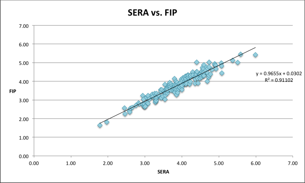
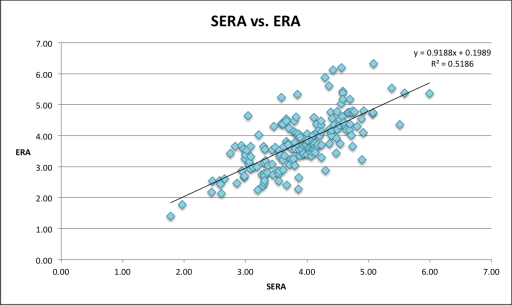
Which makes sense, because what’s going into FIP is also going into SERA. There are, however, some pitchers whom SERA likes a lot more than FIP does…

• Edinson Volquez
• Alex Cobb
• Chris Young
• Danny Duffy
• Clay Buchholz

And also those whom FIP likes more:

• Edwin Jackson
• Masahiro Tanaka
• Ervin Santana
• Brandon McCarthy
• Tim Lincecum
• Adam Wainwright
• Hyun-Jin Ryu
• Phil Hughes
• Stephen Strasburg…

This list goes on much longer than that; generally, I think FIP tends to be more favorable towards better pitchers than SERA does, and specifically I think it is more favorable to low-walk pitchers (maybe we are overstating the negative impacts of walks? Worth thinking about). The average SERA among the pitchers in my 173-count sample was 3.89; for FIP it was 3.79 and for ERA 3.77. We can chalk some of the differences up to random variation in the simulation, because each simulation that gets run is going to be different, but over such a large sample (86.5 million total IP simulated), the difference can’t be all chance. For pitchers who have a large ERA-FIP divide, their SERA almost always comes between the two. The pitchers who had the largest split and didn’t have their SERA fall between their ERA and FIP were:

• Miguel Gonzalez (SERA lower than both)
• Carlos Villaneuva (lower)
• Robbie Ross (lower)
• Josh Beckett (lower)
• Justin Masterson (lower)
• Clay Buchholz (lower)
• Nathan Eovaldi (lower)
• Dan Otero (higher)
• Henderson Alvarez (higher)
• Alfredo Simon (higher)

All but Villaneuva and Ross are pitching, or pitched at one point in their careers, on the East Coast, which can’t possibly be a coincidence and must have some sort of meaning. But other than that, there’s no real obvious explanation. I would guess that there’s no underlying trend here (coastal sea breeze aside), and that this is all random.

Also for reference, here are the year-to-year correlations (r) for pitchers for each of SERA’s components (obtained with the article linked to earlier):

K%	BB%	HR%	GB%	FB%	LD%	IFFB%
0.74	0.59	0.28	0.77	0.76	0.13	0.23

I think this table reinforces the fact that this simulator is more descriptive than it is predictive, just as FIP is. HR%, LD%, and IFFB% all have pretty low year-to-year correlations, meaning that a pitcher with, for example, a high LD% one year will have a low one the next year nearly as likely as a high one. Again, I plan on looking into the predictive capabilities of this model and how it can be adjusted to become more predictive.