FanGraphs Prep: Build and Test Your Own Projection System
This is the third in a series of baseball-themed lessons we’re calling FanGraphs Prep. In light of so many parents suddenly having their school-aged kids learning from home, we hope is that these units offer a thoughtfully designed, baseball-themed supplement to the school work your student might already be doing. The first and second units can be found here and here.
Overview: A two-week unit centered around building and testing your own projection system.
From the simplest forecasts to the most complex projection systems, one of the most challenging questions to try to answer with statistics is predicting player performance from one year to the next. We do this by using their past stats to create an estimate for their future performance. Accounting for other factors like age and injury adds complexity, though not necessarily accuracy. In this unit, you’ll create a simple projection system and then test its accuracy.
Learning Objectives:
- Identify and apply a weighted mean.
- Gather and organize data from various sources.
- Construct a weighted projection using historical data.
- Explain why a projection system produces errors.
- Identify and apply Mean Absolute Error.
- Identity and apply Root Mean Square Error.
- Evaluate which projection error to use for a given problem.
- Review a projection system and adjust to fit data.
Target Grade-Level: 9-10
Daily Activities:
Day 1
Projection systems can get very complex as you take more and more factors into account. But even the most basic projection can still be useful. The Marcel the Monkey Forecasting System is the most basic projection system used in baseball. It’s simply a weighted mean of the past three years of data, age-adjusted, and regressed towards the mean. First, let’s find out how to calculate a weighted mean. A regular mean weighs each input equally. For example:
(2 + 4 + 6 + 8) / 4 = 5
But what if we want to give more weight to one of the inputs. Let’s say the third input is three times as important as the others. To find the weighted mean, we change our example to look like this:
(2 + 4 + (6 * 3) + 8) / 6 = 5.333
It’s important to note that the denominator changed when we changed the weights of the inputs. In our example, the weights of the first, second, and fourth inputs remained 1 but the third input was multiplied by 3. So the sum of our weights is 6, which is what we divide by to get to our weighted mean. This can be written out in an equation:
or multiply the weight (w) of each input (x), sum it all up, and divide by the sum of the weights (w).
Practice calculating the weighted mean using these sample problems.
Day 2
Now, let’s see how we can use a weighted mean to build a simple projection system for baseball. We’ll use three years of historical data for our inputs and weigh the data more heavily the more recent it is. Let’s weigh Year 1 five times as heavily, Year 2 three times as heavily, and leave Year 3 as is. Here are Mike Trout’s home run totals from the last three years:
| Year | Year 1 | Year 2 | Year 3 |
|---|---|---|---|
| Home Runs | 45 | 39 | 33 |
| Weight | 5 | 3 | 1 |
If we apply our weighted mean to this data, we can estimate that Mike Trout will hit 41.667 home runs in 2020 (if a full regular season were played).
Select a few of your favorite players and calculate weighted means for some of their stats using the 5, 3, 1 weighting system we used above.
Day 3
Now let’s add a little more complexity. Our example above assumed that each season Mike Trout played had equal value. But in 2017, he hurt his thumb and missed more than a month of games. Should his home run total in that season weigh the same as the other two seasons where he had a full season of plate appearances? No way! First, let’s calculate how many home runs Trout hit per plate appearance by simply dividing his number of home runs by the number of plate appearances in that year. This gives us a Home Run Rate for Trout.
Next, we’ll apply another weight to our original weights using the number of plate appearances Trout accumulated each year. The new equation would look something like this: Σwyx / Σwy.
| Year | Year 1 | Year 2 | Year 3 |
|---|---|---|---|
| Home Runs | 45 | 39 | 33 |
| Plate Appearances | 600 | 608 | 507 |
| HR/PA Rate | 0.075 | 0.064 | 0.065 |
| Weight | 5 | 3 | 1 |
If we apply our new weighted mean to Trout’s home run rate, we can estimate he’ll hit 0.070 home runs per plate appearance. That sounds weird but if you multiply that rate by the number of plate appearances you expect Trout to receive in 2020, we can estimate he’ll hit 42.2 home runs if he gets 600 plate appearances this season.
Calculate rates and add a playing time weight to the same players and data you used in the previous exercise. How did their projections change when you accounted for playing time in your data?
Day 4
The final factor we’re going to account for in our simple projection system is a concept called regression to the mean. Regression is a complicated concept, so we’ll only touch on it briefly here and leave an in-depth look for another lesson. For any given player, it’s more likely they’ll perform closer to the league average than their recent performance might indicate because data tends to cluster around the league average value.
So in our projection system, we’ll add a league regression factor and a weight to our regression.
The league average home run rate in 2019 was 0.0372 HR/PA. Experiment with adding this regression factor to the players and data you used in the previous exercises. What happens when the regression is weighed heavily? What happens if it’s not as heavy?
Day 5
Since a projection system is only a best guess at a player’s future performance, what sorts of things could happen during a season that could lead to a player over or under performing their projection? What factors could you add to your projection system to account for these circumstances?
Day 6
Now that we’ve got a handle on how to build a projection, let’s see learn how to check the accuracy of our projections. This part of the lesson is brought to you by Jared Cross, the designer of the Steamer Projection system.
Suppose we find ourselves looking at the following ZiPS and Steamer 2019 home run projections for five Mets batters:
| Player | ZiPS HR | Steamer HR | Actual HR |
|---|---|---|---|
| Jeff McNeil | 14 | 11 | 23 |
| Robinson Canó | 16 | 22 | 13 |
| Brandon Nimmo | 13 | 15 | 8 |
| Yoenis Céspedes | 20 | 5 | 0 |
| Todd Frazier | 21 | 14 | 21 |
We would like to determine which set of projections was the most accurate. How should we do it?
Perhaps, most simply, we could look at how many “wins” each projection system has. In this case, it turns out that ZiPS was more accurate for four players (McNeil, Canó, Nimmo and Frazier) whereas Steamer only “won” Céspedes. ZiPS goes 4-1!
I might be tempted to dig a little deeper because my evaluation has a shortcoming – we only looked at numbers of wins and losses and not how decisive they were. Maybe ZiPS’ narrow win on Nimmo shouldn’t count as much as Steamers’ rollicking victory on Céspedes. Let’s explore a couple of oft used metrics for quantifying the size of projection errors, mean absolute error and root mean square error.
Calculating Mean Absolute Error
Our first step is to calculate what are called residuals. These are the differences between the actual values (in this case the numbers of home runs these Mets hit in 2019) and the predictions (from ZiPS and Steamer). And to make sure the negative residuals don’t cancel out the positive ones, we’ll use the absolute value of our residuals.
Abs. Residual = | actual – predicted |
The mean absolute error (MAE) is simply the mean of these residuals.
| Player | ZiPS HR | Steamer HR | Actual HR | ZiPS Abs. Residual | Steamer Abs. Residual |
|---|---|---|---|---|---|
| Jeff McNeil | 14 | 11 | 23 | 9 | 12 |
| Robinson Canó | 16 | 22 | 13 | 3 | 9 |
| Brandon Nimmo | 13 | 15 | 8 | 5 | 7 |
| Yoenis Céspedes | 20 | 5 | 0 | 20 | 5 |
| Todd Frazier | 21 | 14 | 21 | 0 | 7 |
The good news is that we now have a metric that judges these projections by the size of their errors. The bad news (at least for me) is that ZiPS came out ahead again since smaller errors are better. Let’s try root mean square error!
Calculating Root Mean Square Error
Root mean square error (RMSE) is just like mean absolute error except that we’re going to square the residuals before averaging them. Then we’ll take the square root of this average. We can remember the steps in this algorithm by reading the name backwards (1. Error, 2. Square, 3. Mean, 4. Root).
| Player | ZiPS HR | Steamer HR | Actual HR | ZiPS Sq. Error | Steamer Sq. Error |
|---|---|---|---|---|---|
| Jeff McNeil | 14 | 11 | 23 | 81 | 144 |
| Robinson Canó | 16 | 22 | 13 | 9 | 81 |
| Brandon Nimmo | 13 | 15 | 8 | 25 | 49 |
| Yoenis Céspedes | 20 | 5 | 0 | 400 | 25 |
| Todd Frazier | 21 | 14 | 21 | 0 | 49 |
This time, Steamer comes out of top with a smaller root mean square error. You can see why this happened by looking at the squared residuals in the table above. While in our mean squared error calculation, the large Céspedes error was fairly costly, in the root mean square error calculation, ZiPS’ overwhelms the other errors. Root mean square error punishes forecasts for their largest errors.
Day 7
So which metric should we use, MAE or RMSE? It depends. To develop some intuition for what these metrics do, let’s imagine standing in a hall with three elevators at locations 0, 2 and 10.
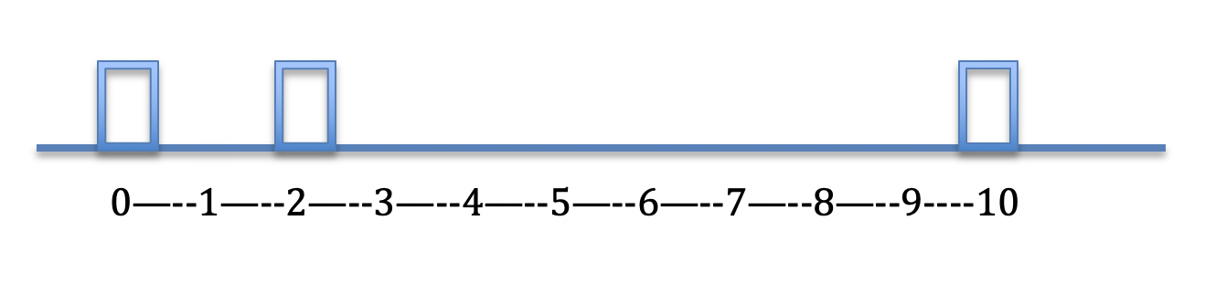
We don’t have any information about which elevator will arrive next but, whichever comes, we’d like to position ourselves to hop on. Where should we stand? Again, it depends.
The place where we choose to stand in this case is essentially our projection for the location of the next elevator. The best choice of location depends on how we evaluate our errors. Our choice of metric ends up being quite important! It determines where we should stand.
- Determine the best place to wait for the elevator in order to minimize our mean absolute error. In other words, where should we stand if we want to minimize the average distance we have to walk to the whichever elevator arrives?
- Determine the best place to wait for the elevator in order to minimize our root mean square error. Where should we stand if we want to minimize the squared walking distance?
(Hint: This problem can be solved through trial and error but those who know calculus can use it. If you haven’t encountered calculus but know how to find the vertex of a parabola, that could be useful too!)
Can you generalize your answers to these problems? In other words, what is special about the locations you found? Can you devise short cut methods of finding the best place to stand in order to minimize the mean absolute error and root mean square error that would work for any number of elevators at any positions?
Day 8
Let’s take everything we’ve learned during this unit and put it all together. We’ve put together a spreadsheet that includes data from the last four seasons. Make sure to make a copy of the spreadsheet so that you can edit the data within.
We’ve already applied a weighted mean to the data from 2016–2018 and tested that projection against the data from 2019 using MAE and RMSE. We’ve also provided a section where you can change the weights of each year to see how the errors change. Play around with the weights to see if you can reduce the size of the errors. You also have the ability to change the weight of the regression towards the mean. What happens to the errors when you change this weight?
Day 9
What do these problems tell us about when to use mean absolute error and when to use root mean square error? For instance, if we built a model to project the number of days a player would spend on the IL, which metric might we want to use to evaluate it? If we worked for a player agent and, on behalf of our clients, created a model to project career earnings, which metric might we want to use?
Adaptations for younger or older learners:
To increase complexity:
- Add additional factors to the projection system you build in the first activity. Devise a way to add a factor for age or injury status to your projection.
- Add more stats to the final activity. The spreadsheet in the final activity includes a projection for a single stat. Add additional stats to the spreadsheet to build a more complete projection for a batter and a pitcher.
To decrease complexity:
- Skip the exercises for MAE and RMSE and simply focus on building a weighted mean. Learning how to calculate a weighted mean is a really useful skill. Focus on other real world applications for using this concept.
Jared Cross is a co-creator of Steamer Projections and consults for a Major League team. In real life, he teaches science and mathematics in Brooklyn. Jake Mailhot is a contributor to FanGraphs. A long-suffering Mariners fan, he also writes about them for Lookout Landing. Follow him on Twitter @jakemailhot.
For someone who is trying to get better at modeling and, like most people, is stuck indoors, this is a perfect summer project. Thanks for this!