FanGraphs Prep: Regression Towards the Mean
This is the sixth in a series of baseball-themed lessons we’re calling FanGraphs Prep. In light of so many parents suddenly having their school-aged kids learning from home, we hope is that these units offer a thoughtfully designed, baseball-themed supplement to the school work your student might already be doing. The first, second, third, fourth, and fifth units can be found here, here, here, here, and here.
Overview: A one-week unit centered around understanding the concept of regression to the mean. This can be a difficult concept to grasp but it’s important for any aspiring statistician to understand.
Learning Objectives:
- Explain the difference between “true talent” and a statistic.
- Use algebra to calculate probabilities.
- Estimate future performance using a projection.
- Identify and apply Regression to the Mean.
Target Grade-Level: 9-10
Daily Activities:
Day 1
Strat-O-Matic is a two-player card-based baseball game. You start by making lineups and then play out a series of batter-pitcher matchups like the one below between Mike Trout and Clayton Kershaw.
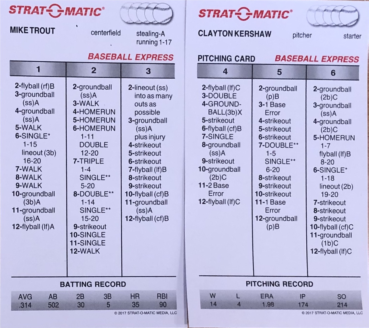
Each matchup involves rolling three six-sided dice. The first one tells you which column to use and the next two determine the outcome, although sometimes we will need to roll an additional 20-sided die. For instance, if the first die roll is a 1, we’ll direct our eyes to the left-most column on Trout’s card. If the next two dice add up to 7, Trout has worked a walk.
Trout’s card determines exactly how good he is in this game. Even if Strat-O-Matic Trout was on a miserable 2-for-50 stretch, I would know that I don’t need to give him a day off to think it over because his card has not changed. In fact, in Strat-O-Matic, I would never make any decisions based on a player’s outcomes in the game, because they don’t change what’s on the card and the card is all that matters. I call Trout’s card his “true talent.” In real life, we never get to see these cards. We might imagine that they exist – that Trout has some underlying level of ability that determines his results, even if his real life card would need to be much more complex and might change subtly day-to-day or even from one moment to the next. Real life Trout’s precise “true talent” is forever unknowable. What we observe are Trout’s statistics, but his statistics are useful only to the extent that they help us estimate his true talent. Simply put — maybe too simply — this is what statisticians do. They observe statistics and then make inferences about unknowable parameters. We see Trout’s results and speculate about his ability.
Sometimes the language we use obscures whether we’re talking about a parameter or a statistic. If I say that Gerrit Cole is the best pitcher in baseball, perhaps it seems like I’m making a statement about his true talent (a parameter). But what if I say that Cole was the best pitcher in baseball last year? Am I simply claiming that he had the best results (statistics) or that he had the most underlying ability over that span of time?
Is it a parameter or a statistic?
For each of the following statements, state whether you think it describes an estimated parameter (“true talent”) or is a statistic.
- Juan Soto hit 34 home runs last year.
- Juan Soto has a .393 career wOBA.
- Juan Soto has a 40% chance of reaching base every time he comes to the plate.
- Juan Soto has 8.5 career WAR
- When Juan Soto attempts a stolen base, he has an 80% chance of success.
Questions to think about:
Does it mean something different to say that someone was the best player than it does to say that they were the most valuable player? Do you think that these are statements about parameters or about statistics?
You may be familiar with some of the following pitching metrics: FIP, xFIP, SIERA, DRA, kwERA. Do you see these metrics as attempts to estimate a pitcher’s true talent or attempts to estimate the quality of his performance? Is there a difference?
Day 2
How long might it take to find the difference between Mookie Betts and Kevin Pillar?
Let’s pretend that the center fielder for my favorite team is either Mookie Betts or Kevin Pillar but that, for some reason that will remain mysterious, I don’t know which. Let’s further pretend that my only avenue for discovering this center fielder’s true identity involves looking up his wOBA on FanGraphs. How long might this mystery last?
In an attempt to find out, let’s create simple Strat-O-Matic cards for Mookie Betts and Kevin Pillar. We’ll use their 2020 Steamer Projections as estimates of their “true talent.” Keep in mind that we’re pretending here. We don’t ever get to know their actual true talents but we can pretend that we know them and see how things might play out in this fictional universe. I’m also going to skip past figuring out how to assign die rolls to batting outcomes and just assign percentages to outcomes. Here’s what that looks like.
| Statistic | Pillar | Betts | wOBA value |
|---|---|---|---|
| uBB% | 3.8 | 11.2 | 0.69 |
| HBP% | 1.2 | 0.8 | 0.72 |
| ROE% | 0.9 | 0.9 | 0.89 |
| 1B% | 16.2 | 13.5 | 0.87 |
| 2B% | 6.0 | 5.6 | 1.22 |
| 3B% | 0.3 | 0.5 | 1.53 |
| HR% | 3.0 | 4.6 | 1.94 |
| Out% | 68.5 | 62.9 | 0.00 |
| wOBA | 320.3 | 373.9 | N/A |
We see that, in this universe, Betts is much more likely to draw an unintentional walk (11.2% to 3.8%) and Pillar is more likely to make an out (68.5% to 62.9%).
The third column shows the wOBA values for each event. For each batter, you can multiply the percentages by the wOBA values, and add up all of those products to calculate a player’s true talent wOBA. In Mookie Betts’ case that means:

(Note: These wOBA are a bit higher than the FanGraphs equivalents since we’re giving credit for reaching base on errors.)
Now let’s have our imaginary players take some imaginary trips to the plate. If a player steps to the plate three times and singles, walks, and makes an out, his wOBA would be: (0.87 + 0.69 + 0) / 3 = .520
What is a player’s wOBA if he has three singles in three plate appearances? What is a player’s wOBA if he has a double, a home run, and an out in three plate appearances? We can use the “true talent” probabilities shown above to calculate the chance that each player would have any possible wOBA after three times to the plate. What is the probability that Pillar hits three home runs in three plate appearances?
Pillar has a 32.2% (.685 x .685 x .685 = .322) chance of making three straight outs whereas Betts has only a 24.9% (.629 x .629 x .629 = .249) chance. Getting back to our original question (finally!), if our mystery player makes three straight outs, we can now say that there is a 56.3% (.322 / (.322 + .249) = .563) chance that it is Kevin Pillar rather than Mookie Betts.
If our player gets on base three straight times, what is the chance that it’s Mookie Betts?
The distributions of possible wOBAs looks quite a bit different after 50 PA. Now, extreme wOBAs are less likely and wOBAs in the neighborhood of each player’s true talent wOBA are more likely.


After 50 PA, Betts has a 2.40% chance of having a wOBA between .370 and .375 and Pillar has a 2.05% chance of having a wOBA in that range. Therefore, if our mystery player has a wOBA between .370 and .375 after 50 PA, there is a 53.9% (.024 / .024 + .0205 = .539) chance that it’s Mookie Betts.
After 50 PA, Betts has a 4.65% chance of having a wOBA between .400 and .410, and Pillar has a 2.70% chance of having a wOBA in that range. If our mystery player has a wOBA between .400 and .410 after 50 PA, what is the chance that it’s Mookie Betts? What kinds of performances would lead us to believe that our mystery player is Pillar? What kinds of performances do you think would make us more certain about who our mystery player is?
Day 3
Projecting our mystery player
Now imagine that after observing 50 plate appearances that we want to project our mystery player’s performance going forward. We figured out yesterday that if our mystery player wOBA’d between .370 and .375 in 50 PA, there’s a 53.9% chance that it’s Mookie Betts (and a 46.1% chance that it’s Kevin Pillar). There’s therefore a 53.9% chance that our player will hit like Betts going forward (meaning with a “true talent” 0.374 wOBA) and a 46.1% chance that they hit like Pillar (with a “true talent” 0.320 wOBA). We can forecast their performance going forward as a weighted average of these two possible performances (.539 x .374 + .461 x .320 = .349).
We also found out yesterday that after 50 PA, Betts has a 4.65% chance of having a wOBA between .400 and .410 and Pillar has a 2.70% chance of having a wOBA in that range. If our mystery player has a wOBA between .400 and .410 after 50 PA, what performance should we forecast going forward?
A full 2020 season
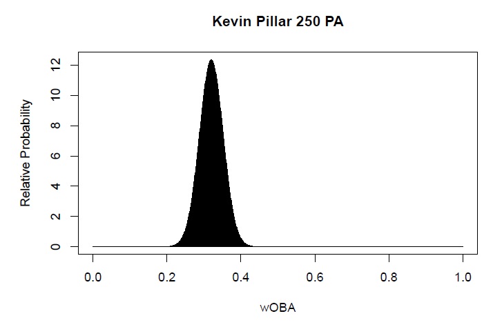
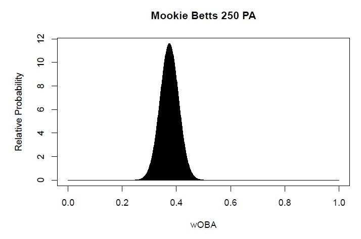
In 60 games, we might expect a regular player to step to the plate something like 250 times. Is that long enough to tell the difference between Mookie Betts and Kevin Pillar? Here are plots showing the relative probability of different wOBAs after 250 PAs for Betts and Pillar. For the sake of saving computational time, we’ve smoothed out the results (assuming a normal distribution) instead of calculating all of the probabilities exactly.
After 250 PA, Mookie Betts has a 5.8% change of having a wOBA between .370 and .375 and Kevin Pillar has a 1.7% chance of having a wOBA in that range. If our mystery player has a wOBA between .370 and .375, what is the probability that they’re Mookie Betts? If our mystery player has a wOBA between .370 and .375 after 250 PA, what wOBA do we project for him going forward?
What if our mystery player could be anyone?
Instead of imagining a universe in which our mystery player can only be Mookie Betts or Kevin Pillar, let’s imagine that all we know is that we’re looking at a major league position player. Once again, I’ll use Steamer as a stand-in for the true talents of these players since their actual talents are unknown. Here’s the distribution of “true talent” wOBAs for 313 regular players.

In this Steamer universe, players have a mean “true talent” wOBA of 0.335. For every one of these 313 players, we can find a distribution of possible wOBAs after 250 PA and, for each player, we can find the chance that the player would have a wOBA between .370 and .375 after 250 PA.
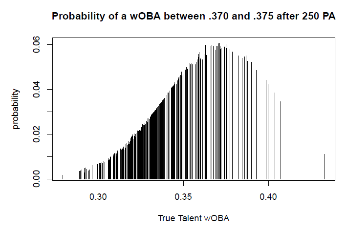
In the graph above each line is one player’s chance of hitting between .370 and .375 after 250 PA. Some batters have somewhat more “boom or bust” profiles but in general, to the surprise of perhaps no one, batters with “true talent” closer to the .370 to .375 range have greater probabilities. The line on its own to the far right represents Mike Trout. Notice that the lines are packed more densely in the neighborhood of .335, the population mean. There are more players with talents closer to average and, as we’ll see, their probabilities will add up.
We can now figure out the chance that our mystery player is any one of these 313 players, the same way we did for Pillar and Betts – we take the probability that a player would have a wOBA in this range and divide it by the sum of the probabilities for all players. Betts, with a 0.6% chance of being our mystery player, is much more likely to be our mystery player than Mike Trout (0.1% chance) or Lewis Brinson (0.02% chance), both of whom are unlikely to have a .370 to .375 wOBA for opposite reasons. We can also forecast our mystery player’s performance going forward the same way we did above. We take a weighted average of true talents of these players, weighing each player by the chance that he’s our mystery man. It turns out that we should project our mystery player to hit 0.347 going forward. We expect an above average performance, but not nearly as strong of one as we’ve seen thus far.
We can repeat this experiment with every player getting 600 PA. After 600 PA, someone like Mookie Betts is far more likely to have a wOBA between .370 and .375 than either Lewis Brinson or Mike Trout.

Repeating the same mathematics as before, we find that after 600 PA of a .370-.375 performance, we’d project our mystery hitter to have a .356 wOBA going forward. Rather than repeating this for every possible performance and number of plate appearances we can use a short hand that works quite well. To project the performance of our unknown hitter going forward, we can just add 450 PA of league average performance (.335 wOBA in
our case) to the performance we observed. Note that this number of plate appearances would be different for different populations of players and for different statistics. For instance, for a player who hit .375 wOBA in 250 PA, we would project ((.375 x 250 + .335 x 450) / (250 + 450) = .349) going forward.
If a hitter had a .450 wOBA in 50 PA, what would we project going forward? If a hitter had a .300 wOBA in 700 PA, what would we project going forward? How would you describe in words how our projections relate to a player’s performances?
The idea of identifying a mystery player from a pool of possible players using only their wOBA is, of course, ridiculous and contrived. But, in reality, we’re often doing something mathematically equivalent. We’re trying to identify a player’s true talent from a distribution of possible talents. Mathematically, we can do the same thing. We take the player’s performance, add in a certain amount of league average performance, and get a better estimate of this player’s true talent. This tells us how he is most likely to perform going forward.
Day 4
Results = Talent + Luck
The upshot is that we always expect players who have performed spectacularly to perform well but not as well going forward and, conversely, the worst performers are expected to be subpar but better than they’ve been. We can understand this by realizing that a player’s results are a combination of their talent and, for lack of a better term, luck. Players with great results are both likely to be above average and likely to have had above average luck. Now, exceptions are certainly possible! A player with great results could have done so despite bad luck thus far and be even better than we imagine! But that’s not the most likely explanation. Since good luck increases the chances of good results, good results are more likely to come from the lucky than the unlucky.
We can state this principle even more generally as: Measurement = True Value + Noise
Any time we observe something and make a measurement, that measurement comes with error or “noise.” Even when we make straight forward measurements — for instance, when we each measure our respective daughters’ heights — the results reflect the “truth” along with some measurement error. If we observe our daughters to be taller than we expected, our measurement was more likely to have erred in the tall direction and our best guess would be that they are in fact a bit shorter than our measurements suggest. The better we are at measuring heights, the less of an adjustment we should apply.
This idea of taking our observations and hedging them, to some extent, in the direction of our expectations is what we call regression towards the mean. Regression towards the mean is a phenomenon that pertains to all imperfect measurements (which is essentially all measurements). The more noise/measurement error/luck is involved in our measurement, the more regression towards the mean there will be. 50 PA and 600 PA both provide imperfect measures of a batter’s ability, but a 50 PA sample is much nosier. As a result, we will regress a 50 PA performance further towards the mean.
Regression towards the mean in practice
Let’s look at the 98 batters who had enough PA to qualify for the leaderboards in both the first and second half of the 2019 season. These hitters had an average wOBA of .345 in each half. Here are the top 10 wOBAs from the first half of 2019:
| Name | wOBA |
|---|---|
| Cody Bellinger | .448 |
| Charlie Blackmon | .414 |
| Peter Alonso | .410 |
| Anthony Rendon | .404 |
| Freddie Freeman | .403 |
| Kris Bryant | .399 |
| Carlos Santana | .398 |
| Juan Soto | .394 |
| Rhys Hoskins | .389 |
| Jeff McNeil | .389 |
These players averaged a .405 wOBA in the first half of 2019. How do you think they did in the second half?
| Name | 1st Half wOBA | 2nd Half wOBA |
|---|---|---|
| Cody Bellinger | .448 | .371 |
| Charlie Blackmon | .414 | .356 |
| Peter Alonso | .410 | .353 |
| Anthony Rendon | .404 | .421 |
| Freddie Freeman | .403 | .365 |
| Kris Bryant | .399 | 0.351 |
| Carlos Santana | .398 | .357 |
| Juan Soto | .394 | .394 |
| Rhys Hoskins | .389 | .293 |
| Jeff McNeil | .389 | .379 |
These players averaged a wOBA of .364 in the second half – still well above average but a far cry from their performance in the first half. Did they get worse? No! Or at least, not necessarily. Regression towards the mean argues that they simply weren’t as good as they appeared in the first half, a half that included above average luck. We see the same thing if we look at the bottom 10 hitters from the first half:
| Name | 1st Half wOBA | 2nd Half wOBA |
|---|---|---|
| Starlin Castro | .259 | .365 |
| Brandon Crawford | .272 | .291 |
| Rougned Odor | .275 | .329 |
| Yolmer Sánchez | .281 | .281 |
| Kevin Pillar | .285 | .312 |
| Lorenzo Cain | .287 | .326 |
| Mallex Smith | .288 | .264 |
| Willy Adames | .293 | .339 |
| Orlando Arcia | .297 | .229 |
| Jose Iglesias | .297 | .317 |
These 10 hitters averaged a .283 wOBA in the first half and then a .305 wOBA in the second half. As a group, they were unlucky in the first half and that’s part of what placed them in the bottom 10. There’s nothing special about wOBA, baseball, or even sports here. If we take the top performers in any sample, we can expect to find that they did worse (but still above average) in another sample. The bottom performers can be expected to collectively do better.
Perhaps counter intuitively, this does not mean that everyone becomes more average over time and the day will come when there are no standout performances. Our expectation for any individual is that they will be more average than they’ve been but there will be enough variance around our expectations that the performances of the population as a whole will remain just as varied going forward as they have been. To circle back to Day 1, regressions towards the mean only applies to “statistics.” We would not expect “true talent” to regress towards the mean. Regression towards the mean is a byproduct of the fact that statistics don’t perfectly reflect true talent.
Day 5
Why we’re punished for praise, sophomore slumps and the Sports Illustrated cover jinx
Psychologist Daniel Kahneman wrote:
“I had the most satisfying Eureka experience of my career while attempting to teach flight instructors that praise is more effective than punishment for promoting skill-learning. When I had finished my enthusiastic speech, one of the most seasoned instructors in the audience raised his hand and made his own short speech, which began by conceding that positive reinforcement might be good for the birds, but went on to deny that it was optimal for flight cadets. He said, “On many occasions I have praised flight cadets for clean execution of some aerobatic maneuver, and in general when they try it again, they do worse. On the other hand, I have often screamed at cadets for bad execution, and in general they do better the next time. So please don’t tell us that reinforcement works and punishment does not, because the opposite is the case.”
This was a joyous moment, in which I understood an important truth about the world: because we tend to reward others when they do well and punish them when they do badly, and because there is regression to the mean, it is part of the human condition that we are statistically punished for rewarding others and rewarded for punishing them. I immediately arranged a demonstration in which each participant tossed two coins at a target behind his back, without any feedback. We measured the distances from the target and could see that those who had done best the first time had mostly deteriorated on their second try, and vice versa. But I knew that this demonstration would not undo the effects of lifelong exposure to a perverse contingency.”
Regression towards the mean, while nearly a law of the universe, still catches us off guard and risks causing us to believe things that aren’t so. In baseball, we talk about sophomore slumps and the home run derby curse but in truth, we should expect the first year players with the most spectacular performances to disappoint the following year and the players with the most home runs in the first half of the season to drop off in the second half. Likewise, players who have performed spectacularly enough to find their way onto a Sports Illustrated cover would be expected to come down to Earth with or without a jinx. More seriously, failing to account for regression towards the mean might cause us to overestimate the effectiveness of medical treatments.
Baseball analysts need to be wary of regression towards the mean at every turn. If we’re concerned with how baseball players age, we should be aware that players who performed better in one year are more likely to get the chance to play again and that these players, as a group, are likely to perform somewhat worse going forward without an aging effect. If we’re interested in how starting pitchers perform in relief, we should be aware that the pitchers who have struggled as starters are more likely to get bumped into relief roles and that these pitchers would likely perform a bit better going forward without any change in role.
If we’re interested in the difference in talent level between Triple-A and the majors, and we look at players who played at both levels in the same season, how might a failure to account for regression towards the mean effect our conclusions?
Adaptations for younger or older learners:
To increase complexity:
- Find a situation from the sports world or otherwise where regression towards the mean may apply, collect data, and see what it reveals.
- Think of a scenario where regression towards the mean may have affected your thinking.
Jared Cross is a co-creator of Steamer Projections and consults for a Major League team. In real life, he teaches science and mathematics in Brooklyn. Jake Mailhot is a contributor to FanGraphs. A long-suffering Mariners fan, he also writes about them for Lookout Landing. Follow him on Twitter @jakemailhot.
As I was reading this I thought, wow, whoever wrote this should be a teacher. Then I reached the end. Jared IS a teacher. Great job, guys.